Hello! Welcome to the fourth lesson in our module on optimization.
In our last lesson, we implemented Batch Gradient Descent, the foundational algorithm for training many machine learning models. We saw how it uses the entire training dataset to compute the gradient of the loss function at each step, ensuring a smooth and steady path towards the minimum.
However, a critical question arises: what happens when "the entire dataset" is enormous? In modern machine learning, datasets can contain millions or even billions of data points. Calculating the gradient across all of them for a single parameter update is incredibly slow and computationally expensive. It's like trying to survey an entire mountain range just to decide which direction to take your next single step.
Today, we'll explore more efficient and practical alternatives. Our learning outcome is to differentiate between batch, mini-batch, and stochastic gradient descent and their trade-offs. We'll see how by adjusting the amount of data we use for each update, we can navigate a trade-off between computational speed and the stability of our descent.
The Problem with Batch Gradient Descent
Let's first solidify our understanding of the computational challenge posed by Batch Gradient Descent when dealing with large datasets.
Stochastic Gradient Descent, Clearly Explained!!!
The video 'Stochastic Gradient Descent, Clearly Explained!!!' from the StatQuest with Josh Starmer channel provides an excellent motivation for why we need alternatives to Batch GD.
Watch from 3:00 to 4:27. Focus on how the number of calculations explodes when you have a large model (many parameters) and a large dataset (many samples). This section clearly sets up the problem we're about to solve.
As you can see, performing trillions of calculations for every single step of the optimization process is not feasible. This computational bottleneck is the primary motivation for the variants of gradient descent we will now discuss.
The Three Flavors of Gradient Descent
The core idea behind the different gradient descent variants is simple: instead of using all the data for each update, we can use a subset. The key difference lies in the size of that subset.
Let's watch a video that introduces and compares all three methods.
Stochastic Gradient Descent vs Batch Gradient Descent vs Mini Batch Gradient Descent |DL Tutorial 14
This video from the codebasics channel provides a clear, side-by-side explanation of Batch, Stochastic, and Mini-Batch Gradient Descent.
Please watch from 0:39 to 7:45. As you watch, focus on answering these questions for each method: Batch GD (0:39 - 2:58): How many samples are used to calculate the error before an update? (You already know this, but it's a good refresher.) Stochastic GD (2:58 - 5:26): How many samples does SGD use? How does this solve the computational problem? Mini-Batch GD (6:01 - 7:16): How does this method find a middle ground between the other two? The summary at 7:16 provides a very concise recap of the main difference.
This gives us a great high-level overview. Now, let's dive deeper and formalize these concepts.
1. Batch Gradient Descent (The "Vanilla" Version)
- How it works: Computes the gradient of the loss function using the entire training dataset for each parameter update.
- Update Rule:
- Pros:
- Stable Convergence: The descent path is smooth and direct because each step is an accurate estimate of the true gradient.
- Guaranteed Convergence: For convex loss functions, it's guaranteed to converge to the global minimum.
- Cons:
- Computationally Expensive: Prohibitively slow and memory-intensive for large datasets.
- Inefficient: Makes very infrequent updates (one per epoch).
2. Stochastic Gradient Descent (SGD)
- How it works: Computes the gradient and updates the parameters using just one randomly selected training sample at a time. An epoch consists of iterating through all samples one by one.
- Update Rule: , for a random sample .
- Pros:
- Fast Iterations: Computation per update is extremely cheap.
- Handles Large Datasets: Can process massive datasets that don't fit in memory.
- Escapes Local Minima: The noisy updates can help the optimizer jump out of shallow local minima.
- Cons:
- High Variance/Noisy Convergence: The loss function fluctuates wildly, and the path to the minimum is very erratic. It never truly settles at the minimum but oscillates around it.
- Inefficient Vectorization: Processing one sample at a time doesn't take advantage of optimized matrix operations in libraries like NumPy or on GPUs.
3. Mini-Batch Gradient Descent (The Practical Choice)
- How it works: This is the compromise. It computes the gradient and updates parameters using a small batch of training samples (e.g., 32, 64, or 256) at a time.
- Update Rule: , for a mini-batch of samples.
- Pros:
- Balanced Approach: Combines the stability of Batch GD with the efficiency of SGD.
- Efficient Computation: Allows for vectorized operations on mini-batches, making it highly efficient on modern hardware like GPUs.
- Smoother Convergence: The loss fluctuates less than in SGD, leading to a more stable convergence.
- Cons:
- New Hyperparameter: Introduces the "batch size" which needs to be tuned.
Visualizing the Convergence Paths
A picture is worth a thousand words when it comes to understanding the behavior of these algorithms.
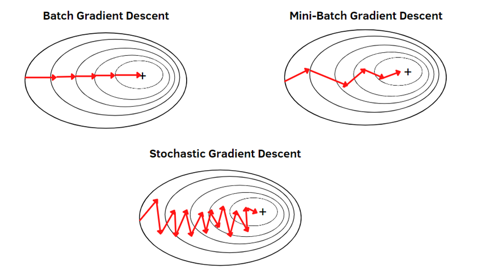
The "zigzag" nature of SGD also shows up when you plot the cost over time. The codebasics video demonstrates this clearly. In SGD, the cost doesn't decrease smoothly; it jumps up and down while trending downwards overall. In contrast, the cost for Batch GD decreases in a much more predictable, smooth curve. Mini-batch would be somewhere in between.
A Comparative Summary
For a final, structured comparison, let's consult a reading that lays out these differences clearly.
Gradient Descent vs. Mini-Batch Gradient ...
The article 'Gradient Descent vs. Mini-Batch Gradient ...' from lunartech.ai provides a detailed comparison that will help solidify your understanding. We will focus on the summary table.
Please read 'Chapter 4: Comparative Analysis – GD vs. SGD vs. Mini-Batch GD'. Pay special attention to the 'Summary Table'. This table directly compares the three methods across the key dimensions: Data Usage, Update Frequency, Computational Efficiency, and Convergence Pattern.
Here is a summary of the key trade-offs:
| Feature | Batch Gradient Descent | Stochastic Gradient Descent (SGD) | Mini-Batch Gradient Descent |
|---|---|---|---|
| Data per Update | Entire dataset | One random sample | A small batch (e.g., 32-256 samples) |
| Update Frequency | Very low (1 per epoch) | Very high (n per epoch) | High (n / batch_size per epoch) |
| Computational Speed | Very slow | Fast | Very fast (due to vectorization) |
| Memory Requirement | High | Low | Low |
| Convergence Stability | Smooth and stable | Noisy, high variance | Relatively smooth, low variance |
| Best For | Small datasets where accuracy is key. | Very large datasets, online learning. | Most practical applications in ML/DL. |
Test your understanding!
You are tasked with training a deep learning model to classify millions of high-resolution images. Your machine has a powerful GPU.
- Which gradient descent variant would you choose?
- Why is your choice the most suitable for this scenario?
- What are the primary disadvantages of the other two variants in this context?
Show answer
-
You would choose Mini-Batch Gradient Descent.
-
It is the most suitable because:
- The dataset is too large for Batch Gradient Descent to be feasible; it wouldn't fit in memory and would be incredibly slow.
- Mini-Batch GD allows you to leverage the parallel processing power of the GPU through vectorized operations on each batch, making it highly efficient.
- It provides a good balance of stable convergence and computational speed.
-
The disadvantages of the others are:
- Batch GD: It would be computationally prohibitive. Each update step would require processing millions of images, taking an enormous amount of time and memory.
- Stochastic GD: While fast per-sample, it fails to fully utilize the GPU's parallel processing capabilities. Processing one image at a time is inefficient compared to processing a batch of 64 or 128 images simultaneously. The convergence would also be very noisy.
Conclusion
In this lesson, we dissected the family of gradient descent algorithms. You learned that while Batch Gradient Descent is conceptually simple and stable, its computational cost makes it impractical for the large datasets common in modern machine learning.
Key Takeaways:
- Batch Gradient Descent: Uses the entire dataset for each update. It's stable but slow.
- Stochastic Gradient Descent (SGD): Uses a single sample per update. It's fast but has a noisy, erratic convergence.
- Mini-Batch Gradient Descent: Uses a small batch of samples per update. It strikes an optimal balance between computational efficiency (by leveraging vectorization on GPUs) and convergence stability. It is the de facto standard for training neural networks.
- The choice of algorithm involves a fundamental trade-off between the accuracy of the gradient estimate and the speed of computation.
Preview of the Next Lesson:
Regardless of which variant you choose, the learning rate remains a critical hyperparameter that determines the size of each step you take. A poorly chosen learning rate can ruin your training process, causing it to go too slowly, get stuck, or even diverge completely. In our next lesson, we will focus on how to "Diagnose and address issues with learning rates (too high or too low)."