Optimizing Learning Rates

What is the Learning Rate, Again?

As a quick recap, the learning rate is the "step size" we take in the direction opposite to the gradient. It scales the gradient to determine the magnitude of the update to our model's weights in each iteration.

The update rule we've been using is:

Here, $\alpha$ directly controls how large of an update we make.

The key takeaway is that this small number has a massive impact on the training process. Let's see what happens when we get it wrong.

Diagnosing Learning Rate Issues from Loss Curves

The most powerful tool for diagnosing learning rate problems is the loss curve, which plots the loss value at each epoch or iteration. The shape of this curve tells a story about how your model is learning.

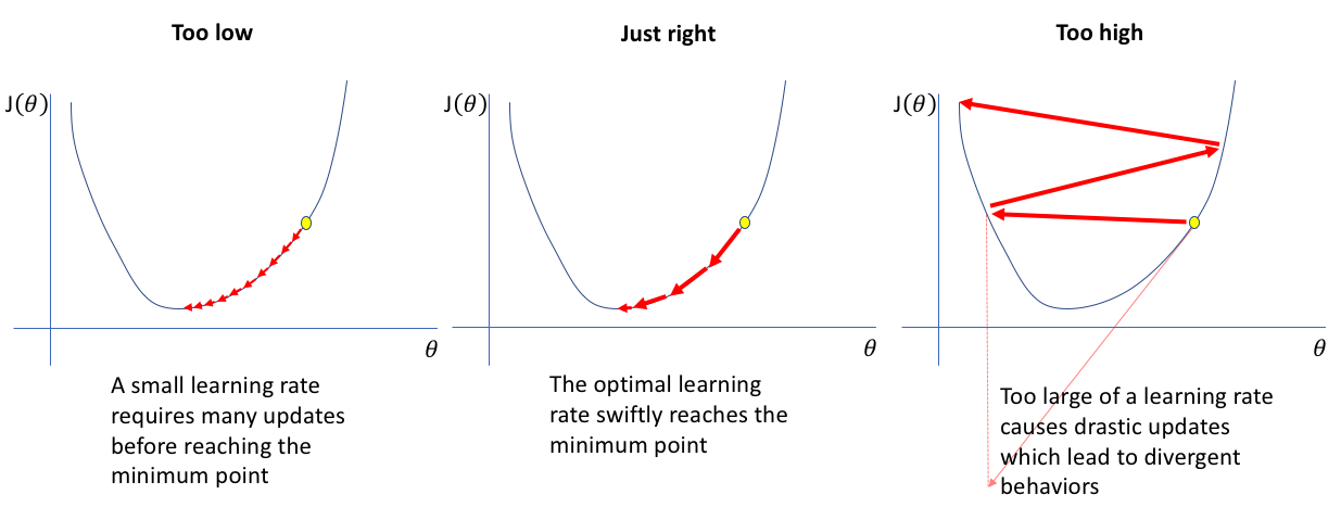
Let's break down how these scenarios manifest in the loss curves you'll see during training. The article "Interpreting Learning Curve Patterns" from the Hugging Face LLM Course provides excellent visual examples.

Based on the reading and the image above, we can summarize the key symptoms:

1. Learning Rate is Too High

• Symptom: The loss doesn't decrease. It might fluctuate wildly, jump around, or even increase, leading to an "exploding" loss (NaN values).
• Why it happens: The steps you're taking are too large. You're overshooting the minimum of the loss landscape and landing somewhere with an even higher loss. The optimization process becomes unstable and diverges.
• What the curve looks like: Erratic and spiky, or trending upwards.

2. Learning Rate is Too Low

• Symptom: The loss decreases, but incredibly slowly. The model takes a huge number of epochs to converge, or it may appear to plateau prematurely because the updates are too small to make meaningful progress.
• Why it happens: The steps are too small, leading to extremely slow progress down the loss gradient. It can also cause the model to get stuck in a shallow local minimum, unable to make a large enough step to get out.
• What the curve looks like: The curve is very smooth but almost flat, decreasing at a snail's pace.

3. The Learning Rate is "Just Right"

• Symptom: The loss shows a steady, reasonably steep decline, which gradually becomes less steep as training progresses and the model approaches a minimum.
• Why it happens: The step size is large enough to ensure fast progress but small enough to allow the model to settle in a good minimum.
• What the curve looks like: A healthy, downward-sloping curve that eventually flattens out (converges).

Strategies for Finding and Managing the Learning Rate

Diagnosing the problem is the first step. Now, let's look at how to fix it. We won't just guess and check; there are systematic methods for managing the learning rate.

Let's summarize these powerful strategies.

1. The Learning Rate Range Test (LR Finder)

This is a fantastic technique to find a good initial learning rate. Instead of guessing, you do a quick experiment:

• Start with a very small learning rate (e.g., $10^{-7}$).
• Run your model for one epoch, but on each mini-batch, you exponentially increase the learning rate.
• Plot the loss against the learning rate (on a log scale).

You will get a plot like this:

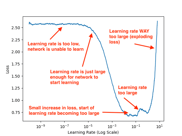
A good rule of thumb is to pick a learning rate from the part of the curve where the loss is decreasing most steeply, for instance, $10^{-4}$ or $10^{-3}$ in the plot above.

2. Learning Rate Schedules

It's often beneficial to change the learning rate during training. A common strategy is to start with a relatively high learning rate for faster initial convergence and then decrease it. This allows the model to take smaller, more precise steps as it gets closer to a minimum, helping it to settle in a more optimal spot. This process is called learning rate decay or annealing.

Common schedules include:

• Step Decay: Reduce the LR by a factor (e.g., 0.1) every N epochs.
• Cosine Annealing: Smoothly vary the learning rate from a high value to a low value following a cosine curve. This is very popular and effective.
• ReduceLROnPlateau: Monitor a metric (like validation loss) and reduce the LR if it stops improving for a "patience" number of epochs.

3. Adaptive Optimizers

As mentioned in the article, optimizers like Adam (which we will cover in detail later) automatically adapt the learning rate for each model parameter. They are much less sensitive to the initial learning rate choice and are often a great default choice, simplifying the tuning process.

Deeper Connections: Why Learning Fails

Sometimes, a learning rate appears to be the problem, but the root cause lies deeper. Your engineering background will appreciate that this is a system with interacting parts. A failure in one component can manifest as a problem in another.

Let's watch a segment from a classic lecture by Andrej Karpathy that explores two critical concepts that are deeply intertwined with the learning rate: weight initialization and batch normalization.

This gives us two profound insights:

1. Bad Initialization Can Mimic a Bad Learning Rate: If your initial weights are chosen poorly, they can cause gradients to become either infinitesimally small (vanishing gradients) or astronomically large (exploding gradients).
   • If gradients vanish, your weights won't update, which looks just like a learning rate that is too low.
   • If gradients explode, your loss will become NaN, which looks just like a learning rate that is too high.
2. Batch Normalization Stabilizes Training: By re-normalizing the activations within the network at every layer, Batch Normalization ensures that gradients are healthier. This makes the optimization process more stable and less dependent on perfect initialization. As a direct result, you can often get away with using a higher learning rate, which accelerates training.

Conclusion

Mastering the learning rate is a mix of science and art, but the techniques we've discussed today move it firmly into the realm of engineering. You now have a systematic toolkit for diagnosing and addressing one of the most common failure points in model training.

Key Takeaways:

• Diagnose via Loss Curves: A flat or slowly decreasing loss suggests the learning rate is too low. An erratic, fluctuating, or exploding loss suggests it's too high.
• Find a Good Starting Point: Use a Learning Rate Range Test to quickly find an optimal range for your initial learning rate, avoiding guesswork.
• Manage the LR During Training: Use learning rate schedules (like Cosine Annealing or Step Decay) to decrease the LR over time, allowing for faster initial training and finer-grained convergence later.
• Consider the Whole System: Remember that issues like poor weight initialization can manifest as learning rate problems. Techniques like Batch Normalization can stabilize training and allow for higher, more effective learning rates.

Preview of the Next Lesson:

While adjusting the learning rate helps control the size of our steps, what about the direction? The noisy gradients from Mini-Batch GD can cause our optimization path to zigzag inefficiently. In the next lesson, we will explore how momentum can help accelerate and stabilize gradient descent, effectively smoothing out the path to the minimum.