Momentum in Gradient Descent

The Problem: Zigzagging Down the Ravine

Imagine the loss function isn't a simple, symmetrical bowl, but a long, narrow valley or ravine. This is very common in neural network loss landscapes.

Standard gradient descent calculates the steepest direction at its current position. On the steep walls of the ravine, this direction points almost directly across the valley, not down the valley floor toward the minimum. As a result, the optimizer bounces from one side of the ravine to the other, making slow progress toward the actual solution. These oscillations force us to use a smaller learning rate to prevent divergence, which slows down convergence even more.

To visualize this issue, let's watch a segment from a video by Andrew Ng.

The key issue is that gradient descent is amnesiac—it only considers the gradient at the current step, with no memory of its past direction. Momentum is the technique we use to give our optimizer this memory.

The Intuition Behind Momentum

The core idea of momentum is to simulate physical momentum. Instead of just following the current gradient, we add a fraction of our previous update vector to the current one.

Think of it like a ball rolling down a hill:

• It doesn't just move based on the slope at its exact current location; it carries velocity from its past movement.
• As it rolls down a consistent slope, it builds up speed.
• This accumulated speed helps it power over small bumps (noise in the gradient) or escape shallow valleys (local minima).

This simple idea has a powerful effect on the zigzag problem:

• In the oscillating direction (across the ravine): The gradients are constantly switching signs (e.g., +0.5, -0.5, +0.5...). When we average them over time, they tend to cancel each other out, damping the oscillations.
• In the consistent direction (down the ravine): The gradients are always pointing in the same direction. When we average them, they reinforce each other, building up speed and accelerating convergence.

To dive deeper into this intuition, the following article offers some excellent analogies.

The Mathematics of Momentum

The "memory" in momentum is implemented using an Exponentially Weighted Moving Average (EWMA) of the gradients. Instead of updating the weights directly with the current gradient, we first calculate a "velocity" vector, $\mathbf{v}$, which is a smoothed average of the gradients, and then use this velocity to update the weights.

Here's how it works at each iteration $t$:

1. Compute the gradients $\nabla J({\theta }_t)$ on the current mini-batch (we'll denote this as $d\theta$).
2. Update the velocity using the EWMA formula:
   ${\mathbf{v}}_t=\beta {\mathbf{v}}_{t-1}+(1-\beta )d{\theta }_t$
   • ${\mathbf{v}}_t$ is the new velocity.
   • ${\mathbf{v}}_{t-1}$ is the velocity from the previous step.
   • $\beta$ is the momentum hyperparameter.
3. Update the parameters using the new velocity:
   ${\theta }_{t+1}={\theta }_t-\alpha {\mathbf{v}}_t$

Notice the key difference: we subtract $\alpha {\mathbf{v}}_t$, not $\alpha d{\theta }_t$. We are moving in the direction of the smoothed average gradient.

Let's watch Andrew Ng explain this formulation.

The Momentum Hyperparameter: $\beta$

The hyperparameter $\beta$ controls the "friction" in our system. It determines how much of the past velocity is carried over to the current step.

• If $\beta =0$, then ${\mathbf{v}}_t=d{\theta }_t$, and we recover standard gradient descent. There is no memory.
• If $\beta$ is close to 1, we consider a long history of past gradients.
• A common and very effective value for $\beta$ is 0.9.

With $\beta =0.9$, the update is roughly averaging over the last $\frac{1}{1-0.9}=10$ gradients. This is usually enough to smooth out noise without being overly influenced by outdated information.

The Benefits and a Key Trade-Off

The two main benefits of momentum are what we set out to achieve:

1. Acceleration: By accumulating gradients in a consistent direction, momentum helps the optimizer move faster toward the minimum.
2. Stabilization: By averaging out noisy, oscillating gradients, it smooths the optimization path and makes training more stable.

A powerful side-effect of this is the ability to navigate tricky parts of the loss landscape. The accumulated velocity can help the optimizer "roll through" flat plateaus (saddle points) where the gradient is near zero, or even "power over" shallow local minima.

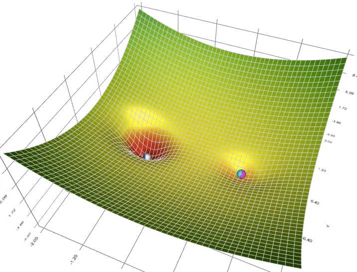
However, momentum's greatest strength—its speed—can also be a weakness.

The Problem of Overshooting:
Because the optimizer has so much momentum, it may not stop precisely at the bottom of the hill. Instead, it can overshoot the minimum, have to reverse, and then oscillate back and forth a few times before it finally settles. While momentum gets you to the vicinity of the minimum much faster, this final settling process can sometimes be tricky.

Conclusion

You now understand one of the most fundamental and effective improvements to the gradient descent algorithm. By adding a "memory" of past updates, momentum transforms the optimization process from a jittery walk into a smooth, accelerating roll toward the minimum.

Key Takeaways:

• Problem: Standard gradient descent is "memoryless" and can get stuck in slow, oscillating paths in the narrow "ravines" of the loss landscape.
• Solution: Momentum uses an exponentially weighted moving average of past gradients to create a "velocity" vector. This update rule smooths out oscillations and accelerates movement in consistent directions.
• Benefits: This leads to faster convergence and more stable training. It also helps the optimizer escape shallow local minima and saddle points.
• Hyperparameter: The momentum term, $\beta$, is typically set to 0.9, which corresponds to averaging over the last 10 gradients.
• Trade-off: The accumulated speed can cause the optimizer to overshoot the minimum before settling.

Preview of the Next Lesson:

Momentum is a huge step forward, but it still uses a single, fixed learning rate, $\alpha$, for all parameters in the model. But what if some parameters need large updates while others need very fine-grained changes? In our next lesson, we will explore adaptive learning rate methods like Adam, which calculate a unique learning rate for every single parameter, combining the ideas of momentum with other clever tricks.