Gradient Descent: Minimizing Loss Iteratively

Hello! Welcome to the second lesson in our module on Optimization for Machine Learning.

In our last lesson, we established the crucial role of a loss function. We learned that it acts as a scorekeeper, quantifying how "wrong" a model's predictions are. This leads to a clear objective for training a model: find the set of parameters (like weights and biases) that minimizes the overall cost function.

This lesson directly addresses the next logical question: how do we find those optimal parameters? We will explore the most fundamental optimization algorithm in machine learning, which answers this question precisely. Our learning outcome is to describe gradient descent as an iterative algorithm for minimizing a loss function. Understanding this process is essential for explaining how most machine learning models, from simple linear regression to complex neural networks, actually learn from data.

The Challenge of Minimization

Imagine a vast, hilly landscape where the elevation at any point represents the value of our cost function for a specific set of model parameters. Our goal is to find the lowest point in this entire landscape—the global minimum.

For simple models, like the ordinary least squares regression you might have seen, we can sometimes solve for this minimum directly using calculus (setting the derivative to zero) or linear algebra (the normal equations). However, for most complex models in machine learning, the "landscape" of the cost function is incredibly complicated, with thousands or even millions of parameters. Solving for the minimum directly becomes impossible.

This is where we need an iterative approach—an algorithm that can start somewhere random and intelligently "walk" downhill until it finds a valley. This algorithm is Gradient Descent.

To get a feel for the scale of this problem and the intuition behind the solution, let's start with a video that frames this in the context of neural networks.

Gradient descent, how neural networks learn | Deep Learning Chapter 2

This video from 3Blue1Brown provides a beautiful conceptual overview of how gradient descent works to minimize a cost function with thousands of parameters, as is common in neural networks.

Please watch from the beginning to 8:27. Focus on these key ideas: The concept of a cost function that measures how 'lousy' the model is. The analogy of finding a minimum by figuring out the 'downhill' direction. How the gradient provides this downhill direction in a multi-parameter space.

The Core Mechanism: Walking Downhill

As the video explained, the core idea is to take small, repeated steps in the direction of the steepest descent. But how do we find this direction? This is where the "guide" role of the loss function comes into play, using a concept from your calculus background: the derivative.

The 1D Case: One Parameter

Let's start with the simplest case: a model with only one parameter, which we'll call $w$ . The cost function, $J (w)$ , is a simple curve.

The derivative, $\frac{dJ}{d w}$ , tells us the slope of the curve at any given point $w$ .
If the slope is positive, it means increasing $w$ will increase the cost. To go downhill, we must decrease $w$ .
If the slope is negative, it means increasing $w$ will decrease the cost. To go downhill, we must increase $w$ .

Notice the pattern: we always want to move in the opposite direction of the slope. This gives us the core update rule for Gradient Descent.

Gradient Descent Intuition with Cost Function Graphs — This image shows how the update rule works. When the slope (derivative) is positive (top), we subtract a positive value from 'w', moving it left. When the slope is negative (bottom), we subtract a negative value, which is equivalent to adding a positive value, moving 'w' right. In both cases, we move towards the minimum.

This leads to the iterative update formula:

w_{new} = w_{old} - α \cdot \frac{dJ}{d w}

Here, $α$ (alpha) is the learning rate, a small positive number that controls how big of a step we take.

Let's watch a detailed, step-by-step example of this process.

Gradient Descent, Step-by-Step

The video 'Gradient Descent, Step-by-Step' from StatQuest is one of the clearest explanations available. It walks through the entire process for a simple linear regression model.

Please watch from 1:56 to 11:25. This section focuses on using gradient descent to find just one parameter (the intercept). Pay close attention to: How the Sum of Squared Residuals is used as the loss function. The calculation of the derivative of the loss function. The role of the learning rate in calculating the 'step size'. How the intercept is updated iteratively, getting closer to the minimum.

Test your understanding!

In the Gradient Descent update rule $w_{new} = w_{old} - α \cdot \frac{dJ}{d w}$ , suppose at your current parameter value $w_{old}$ , the derivative $\frac{dJ}{d w}$ is -2.0. Will $w_{new}$ be greater or smaller than $w_{old}$ ? Does this move you closer to the minimum of the cost function?

Show answer

$w_{new}$ will be greater than $w_{old}$ . The update is $w_{new} = w_{old} - α \cdot (- 2.0) = w_{old} + 2 α$ . Since $α$ is positive, we are adding a positive value.

Yes, this moves you closer to the minimum. A negative derivative means the cost function is sloping downwards as $w$ increases. Therefore, to continue downhill, we must increase $w$ .

The Multi-dimensional Case: The Gradient

Most models have more than one parameter (e.g., both a slope $w_{1}$ and an intercept $w_{0}$ ). Instead of a simple curve, our cost function is now a multi-dimensional surface.

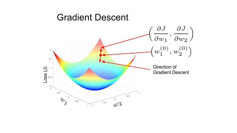
Gradient Descent in 3D — This image visualizes a loss surface for a model with two parameters, w1 and w2. Gradient Descent starts at a random point and iteratively follows the path of steepest descent (the red arrows) to reach the minimum point of the surface (the blue area).

In this multi-dimensional setting, we can't use a simple derivative. Instead, we use the gradient, denoted by $\nabla J$ . The gradient is simply a vector containing the partial derivatives of the cost function with respect to each parameter. For a model with two parameters $w_{0}$ and $w_{1}$ , the gradient is:

\nabla J (w_{0}, w_{1}) = [\frac{\partial J}{\partial w _{0}} \frac{\partial J}{\partial w _{1}}]

Just like the derivative pointed "uphill" on a 2D curve, the gradient vector points in the direction of the steepest ascent on the multi-dimensional surface. To go downhill, we again move in the opposite direction of the gradient.

This gives us the vectorized update rule:

w_{new} = w_{old} - α \cdot \nabla J (w_{old})

This single equation elegantly captures the process of updating all parameters simultaneously. Each parameter is updated according to its own partial derivative, effectively taking a combined step in the direction of the steepest overall descent.

Let's see this in action.

Gradient Descent, Step-by-Step

Let's return to the StatQuest video to see how the process extends to multiple parameters.

Now watch from 15:49 to 21:55. This segment demonstrates: How to calculate the gradient by taking partial derivatives for both the intercept and the slope. How both parameters are updated simultaneously in each step. The concept that gradient descent is sensitive to the learning rate.

The Gradient Descent Algorithm

We can now summarize the entire process into a formal algorithm. This step-by-step procedure is the foundation for how many machine learning models are trained.

Linear regression: Gradient descent

The Google Machine Learning Crash Course provides a very clear, step-by-step summary of the algorithm, along with a concrete numerical example.

Read the first four main sections of this article (up to the table showing loss reduction over iterations). Focus on the four numbered steps that outline the iterative process. Notice how the derivatives for weight and bias are calculated and used to update the parameters.

To summarize the algorithm:

Initialize Parameters: Start by choosing random initial values for your model's parameters ( $w$ ).
Iterate: Repeat the following steps until the model converges:
a. Calculate the Gradient: Compute the gradient of the cost function, $\nabla J (w)$ , at the current parameter values. This involves calculating the partial derivative for every parameter in your model, based on all the data in your training set.
b. Update Parameters: Apply the update rule to get your new set of parameters: $w_{new} = w_{old} - α \cdot \nabla J (w_{old})$ .
Stop: The algorithm has converged when the updates become very small (i.e., the gradient is close to zero, meaning you're at the bottom of a valley) or after a predefined maximum number of iterations.

This standard version of the algorithm, which uses the entire dataset to compute the gradient at each step, is often called Batch Gradient Descent.

Conclusion

In this lesson, we demystified the process of model training by describing Gradient Descent. You now understand the mechanics behind how a model "learns" by iteratively adjusting its parameters to minimize a cost function.

Key Takeaways:

Gradient Descent is an iterative optimization algorithm used to find the minimum of a cost function when a direct solution is not feasible.
The derivative (in 1D) or the gradient (in multiple dimensions) of the cost function provides the direction of steepest ascent.
The core update rule involves taking a step in the opposite direction of the gradient: $w_{new} = w_{old} - α \cdot \nabla J (w_{old})$ .
The learning rate ( $α$ ) is a critical hyperparameter that controls the size of each step.

Preview of the Next Lesson:

We have now described the Gradient Descent algorithm conceptually. The next logical step is to see it in action. In the next lesson, "Implement gradient descent to optimize the parameters of a simple model," we will translate this algorithm into code and use it to train a linear regression model from scratch. This will solidify your understanding by moving from theory to practical application.