The Central Limit Theorem and the Normal Distribution of Sample Means

1. The Core Idea: Order from Randomness

The Central Limit Theorem is a statement about what happens when you take the average of many random observations. In short, it says that regardless of the original population's distribution—be it uniform (like a die roll), exponential (like waiting times), or something completely unknown—the distribution of the sample means will tend to follow a Normal distribution as your sample size gets large enough.

This is a profound result. It implies that a predictable order (the bell curve) emerges from the aggregation of random events.

To build a strong intuition for this, let's watch a video from StatQuest. It demonstrates the CLT visually using different starting distributions.

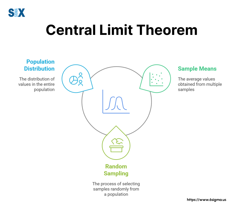
The process described in the video can be summarized in three steps, as illustrated below.

2. A Deeper Look: The Sum of Random Variables

The CLT is often explained in terms of sample means, but it's equally valid for the sum of random variables (since the mean is just the sum divided by the sample size, $n$). Thinking about sums can provide a more fundamental intuition.

Imagine rolling a single die. The outcome is a random variable from a uniform distribution. Now, what if you roll two dice and add their values? The sum is more likely to be 7 than 2 or 12. As you add more and more dice, the distribution of their sum starts to look more and more like a bell curve. Each die roll is an independent, random event, and their aggregation smooths out the randomness into a predictable, normal shape.

The following video from 3Blue1Brown offers a fantastic visual and mathematical intuition for this process.

3. Key Properties and Assumptions

To apply the CLT correctly, we need to understand its properties and the conditions under which it holds.

a) The Sampling Distribution of the Mean

When we repeatedly take samples and calculate their means, the distribution of these means is called the sampling distribution of the mean. The CLT tells us this distribution has two key properties:

1. Mean: The mean of the sampling distribution (${\mu }_{\bar{x}}$) is equal to the mean of the original population ($\mu$).
2. Standard Deviation: The standard deviation of the sampling distribution is called the standard error of the mean (${\sigma }_{\bar{x}}$). It is smaller than the population standard deviation ($\sigma$) and is calculated as:
   ${\sigma }_{\bar{x}}=\frac{\sigma }{\sqrt{n}}$
   where $n$ is the sample size.

This formula is crucial. It shows that as our sample size $n$ increases, the standard error decreases. This means our sample means become more tightly clustered around the true population mean, making our estimate more precise. The Medium article "The Central Limit Theorem and its Role in Data Science" explains this well in the section titled "Variance Shrinks."

b) Necessary Assumptions

The CLT is powerful, but it's not magic. It relies on a few key assumptions about the data.

To summarize, the key assumptions are:

1. Independence: The observations in each sample must be independent of one another.
2. Identical Distribution: All samples should be drawn from the same underlying population distribution. (These first two are often combined and referred to as i.i.d. for "independent and identically distributed").
3. Finite Variance: The population distribution must have a finite variance. This is true for almost all distributions you will encounter in practice.

4. Practical Applications in Data Science and ML

So, why is this theorem so vital for a machine learning engineer? Because it allows us to make inferences about populations using samples, which is the foundation of statistical testing and model evaluation.

For a great overview, I recommend reading the following resource.

As the article mentions, here are two key areas where the CLT is applied:

1. Hypothesis Testing (e.g., A/B Testing): When comparing two models or two versions of a product (e.g., website layouts A and B), we look at a metric like the average click-through rate. The CLT allows us to assume the sample mean of this metric is normally distributed, which lets us calculate p-values and determine if the observed difference is statistically significant or just due to random chance.

2. Confidence Intervals: When we evaluate a model, we might get an accuracy of, say, 92% on our test set. But how confident are we in this number? Because of the CLT, we can treat this accuracy score as a sample mean from a distribution of possible scores. This allows us to calculate a confidence interval (e.g., "we are 95% confident that the true model accuracy is between 91% and 93%"), giving a much better sense of the model's real-world performance.

The Medium article "The Central Limit Theorem and its Role in Data Science" (ID: LINK) provides Python code for these applications under the headings "Confidence Intervals", "A/B Testing", and "Machine Learning Model Evaluation", which I encourage you to explore if you're interested in the implementation details.

Conclusion

Today, you've learned about the Central Limit Theorem, one of the most important concepts in statistics. It provides the crucial link between any population distribution and the predictable, normal distribution of its sample means.

Key Takeaways:

• The What: The CLT states that the sampling distribution of the sample mean will be approximately normal if the sample size is large enough, regardless of the population's original distribution.
• The Why: This happens because summing or averaging many independent random variables smooths out extremes and idiosyncrasies, leading to a symmetric, bell-shaped distribution.
• The How: The sampling distribution will have a mean equal to the population mean ($\mu$) and a standard deviation (standard error) of $\sigma /\sqrt{n}$.
• The Importance: It is the theoretical justification for many statistical inference methods used in machine learning, such as hypothesis testing and constructing confidence intervals.

Next Steps:
So far in this module, we have focused on understanding and modeling single variables. However, in machine learning, we are almost always interested in the relationship between variables. In our next lesson, we will learn how to measure the strength and direction of the linear relationship between two variables using covariance and correlation.