Measuring Linear Relationships: Covariance and Correlation

1. From Variance to Covariance: Measuring Togetherness

You're already familiar with variance, which measures how much a single variable "varies" from its mean. But what if we have two variables, say, height and weight, and we want to know if they vary together? Does a higher-than-average height tend to correspond with a higher-than-average weight?

This is precisely the question that covariance answers. It measures the joint variability of two random variables.

To build an intuition for this, let's watch a short, conceptual video.

As the video explained, the formula for the sample covariance is:
$\text{Cov}(X,Y)=s_{xy}=\frac{{\sum }_{i=1}^n(x_i-\bar{x})(y_i-\bar{y})}{n-1}$

• If for a given data point, both $x_i$ and $y_i$ are above their respective means, the product $(x_i-\bar{x})(y_i-\bar{y})$ will be positive.
• The same is true if both are below their means (negative times negative is positive).
• If one is above its mean and the other is below, the product will be negative.

Summing these products tells us the dominant trend:

• Positive Covariance: Indicates a positive linear relationship (as one variable increases, the other tends to increase).
• Negative Covariance: Indicates a negative linear relationship (as one variable increases, the other tends to decrease).
• Covariance near Zero: Indicates little to no linear relationship.

However, covariance has a major limitation: its magnitude is hard to interpret. For example, a covariance of 100 might be very strong for one dataset but weak for another, depending on the units and scale of the variables. This is where correlation comes in.

2. Correlation: Normalizing for Strength

Correlation is a standardized version of covariance. It gives us a measure of both the direction and the strength of the linear relationship, and its value is always between -1 and 1, making it easily interpretable.

The formula for the Pearson correlation coefficient ($r$) is:
$r_{xy}=\frac{\text{Cov}(X,Y)}{s_x{s}_y}$
where $s_x$ and $s_y$ are the sample standard deviations of X and Y, respectively. By dividing by the standard deviations, we effectively remove the scale dependency of the variables.

Here's a guide to interpreting the correlation coefficient:

• r = +1: Perfect positive linear relationship.
• r = -1: Perfect negative linear relationship.
• r = 0: No linear relationship.
• Values close to 1 or -1 indicate a strong linear relationship.
• Values close to 0 indicate a weak linear relationship.

The following image provides a great visual for what different correlation values look like.

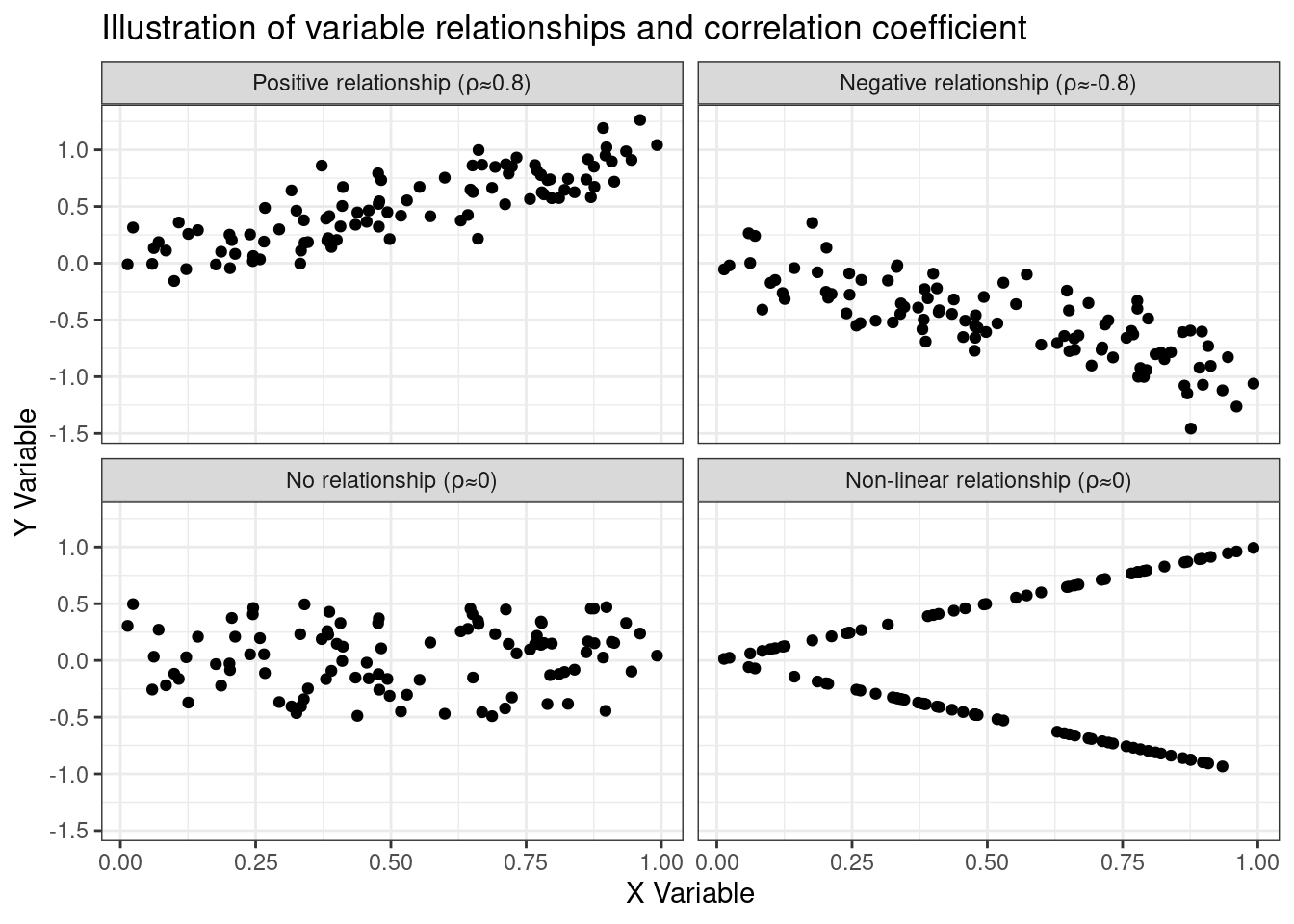
3. Calculating Covariance and Correlation

Now that we understand the concepts, let's walk through the actual calculation. While in practice you'll use software, working through an example by hand is the best way to solidify your understanding of the mechanics.

The following video demonstrates the step-by-step process for a small dataset.

4. Key Considerations for Machine Learning

Understanding how to calculate correlation is the first step. For your goal of applying these concepts in machine learning, it's even more critical to understand its limitations and practical use.

Please read the following document for a consolidated summary and some worked examples.

The resources so far have highlighted two crucial points that every data scientist must remember.

a) Correlation Measures Linear Relationships Only

A correlation coefficient of zero does not mean there is no relationship between the variables; it just means there is no linear relationship. The bottom-right panel of the scatter plot image above shows a perfect quadratic relationship, but its linear correlation is zero. This is a common pitfall. Always visualize your data with a scatter plot before drawing conclusions from a correlation value.

b) Correlation is NOT Causation

This is perhaps the most important maxim in statistics. A strong correlation between two variables does not prove that one causes the other. There could be a third, unobserved variable (a confounding variable) that is influencing both. The reading mentioned the classic example of storks and birth rates being correlated because both are more common in rural areas (the confounding variable).

For a deeper dive into these nuances and to see how to perform these calculations in Python, the primary tool for ML, please review the following article.

As the article shows, you can easily compute the correlation between two variables, X and Y, in Python using NumPy:

import numpy as np

# A matrix is returned, where the off-diagonal elements [0,1] and [1,0]
# contain the correlation coefficient between X and Y.
corr_matrix = np.corrcoef(X, Y)
correlation = corr_matrix[0, 1]

This is the approach you will most often use in practice when exploring a new dataset.

Conclusion

In this lesson, we moved from single-variable analysis to understanding the relationship between two variables. You learned how to quantify this relationship using covariance and correlation, both conceptually and computationally.

Key Takeaways:

• Covariance measures the direction of a linear relationship. Its magnitude is scale-dependent and difficult to interpret.
• Correlation is a normalized version of covariance that measures both the strength and direction of a linear relationship. Its value is always between -1 and 1.
• A correlation of 0 implies no linear relationship, but a non-linear relationship might still exist. Always visualize your data.
• A strong correlation between two variables does not mean one causes the other. Correlation is not causation.

Next Steps:
Today, we looked at the relationship between two variables. In machine learning, datasets almost always contain many more than two features. Our next lesson will generalize today's concepts to the multivariate case. We will learn how to construct and interpret a covariance matrix, a powerful tool for understanding the relationships across all pairs of variables in a dataset at once.