Understanding and Building Covariance Matrices

1. The Anatomy of a Covariance Matrix

Imagine you have a dataset with n features (e.g., age, income, years of education, credit score...). Instead of calculating the covariance for each pair of features one by one, we can organize all this information into a single structure: the covariance matrix.

A covariance matrix (often denoted by the Greek letter Sigma, $\Sigma$) is a square n x n matrix that summarizes the variances and covariances of your n variables.

Its structure is very intuitive:

• The Diagonal Elements: The elements along the main diagonal (from top-left to bottom-right) are the variances of each individual variable. The element in row i and column i is $\text{Var}(X_i)=\text{Cov}(X_i,X_i)$.
• The Off-Diagonal Elements: The elements not on the main diagonal are the covariances between pairs of variables. The element in row i and column j is $\text{Cov}(X_i,X_j)$.

To get a clear visual and conceptual overview of this structure, let's watch the following video.

As the video highlighted, there are two crucial properties to remember:

1. It's a Square Matrix: For n variables, the matrix will have dimensions n x n.
2. It's Symmetric: The covariance between variable X and variable Y is the same as the covariance between Y and X (i.e., $\text{Cov}(X,Y)=\text{Cov}(Y,X)$). This means the matrix is symmetric across its main diagonal. The element at [row i, col j] is identical to the element at [row j, col i].

For a more detailed written explanation of these concepts, you can refer to the following resource.

2. Constructing the Covariance Matrix

Now that we know what a covariance matrix is, let's see how to build one. The process involves calculating the variance for each variable (for the diagonal) and the covariance for each unique pair of variables (for one half of the off-diagonals, since it's symmetric).

Let's watch a complete, worked example for a dataset with three variables.

3. A More Efficient Approach: The Linear Algebra View

Calculating each element individually works, but it's inefficient for datasets with many features. Given your engineering background, you'll appreciate that there's a much more elegant and computationally efficient way to do this using matrix algebra.

If you have a data matrix $X$ where each row is an observation and each column is a feature, the steps are:

1. Center the data: For each feature (column), subtract its mean from every observation in that column. Let's call this new centered matrix $X_c$.
2. Calculate the covariance matrix: The covariance matrix $\Sigma$ can then be calculated with a single matrix operation:

$\Sigma =\frac{1}{m-1}{X}_c^T{X}_c$

where $m$ is the number of observations (samples) and $X_c^T$ is the transpose of the centered data matrix. This formula assumes your data matrix has observations as rows and features as columns, which is the standard convention in libraries like Pandas and Scikit-learn.

The image below provides a great visual summary of this process, though it uses a convention where features are rows and observations are columns. The core idea of using matrix multiplication remains the same.

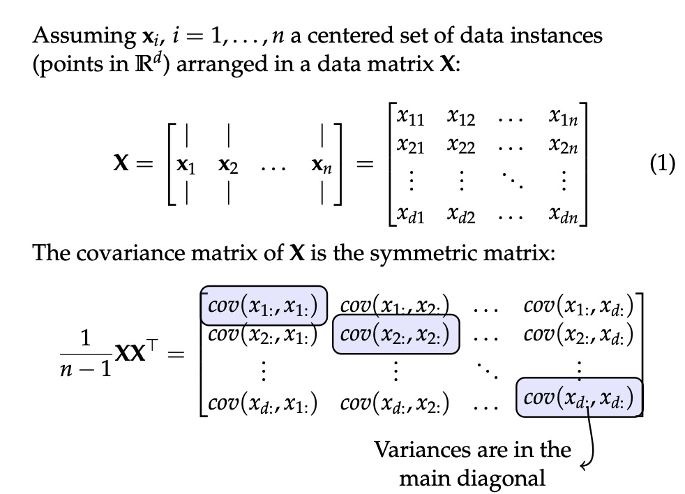
This matrix approach is exactly what libraries like NumPy and Pandas do under the hood. It's significantly faster than looping through pairs of columns.

4. Interpreting the Covariance Matrix

Constructing the matrix is only half the battle. The real value comes from interpreting it to understand the structure of your data.

When you look at a covariance matrix, you should analyze:

• The Diagonal (Variances): These values tell you the spread of each individual feature. A larger value on the diagonal means that feature has a wider range of values.
• The Off-Diagonals (Covariances): These values tell you about the linear relationships between pairs of features.
  • Sign: A positive value means the two features tend to increase or decrease together. A negative value means one tends to increase as the other decreases. A value near zero suggests no linear relationship.
  • Magnitude: This is the trickiest part. The magnitude of covariance is scale-dependent. A large covariance doesn't necessarily mean a stronger relationship; it could just be that the variables themselves have large values and high variance.

The following image clearly illustrates this point. Both plots show a positive correlation, but the scales of the data lead to vastly different covariance values.

Interpretation Example: Stock Portfolio

Let's analyze a practical example from the mlforbeginners.com article. Imagine we have a covariance matrix for the daily returns of three stocks: A, B, and C.

Let's break down what this tells us:

• Variances (Risk):

  • Var(A) = 0.10
  • Var(B) = 0.25
  • Var(C) = 0.15
  • Interpretation: Stock B is the most volatile (riskiest) because it has the highest variance. Stock A is the least volatile.

• Covariances (Relationships):

  • Cov(A, B) = 0.05: Stocks A and B have a positive covariance. They tend to move in the same direction. When Stock A's return is up, Stock B's return also tends to be up.
  • Cov(A, C) = -0.08: Stocks A and C have a negative covariance. They tend to move in opposite directions. This is great for diversification; if Stock A does poorly, Stock C is likely to do well, balancing the portfolio.
  • Cov(B, C) = 0.02: Stocks B and C have a very small positive covariance, suggesting a very weak linear relationship.

5. Calculating the Covariance Matrix in Python

In practice, you will never compute a covariance matrix by hand. Python libraries make it trivial.

Using pandas, which is standard for data manipulation in machine learning:

import pandas as pd
import numpy as np

# Sample data: 3 features, 5 observations
df = pd.DataFrame({
    'Math_Score': [80, 90, 70, 85, 75],
    'Science_Score': [85, 95, 75, 88, 80],
    'Hours_Studied': [10, 15, 8, 12, 9]
})

# Calculate the covariance matrix
cov_matrix = df.cov()

print("Covariance Matrix:")
print(cov_matrix)

And with numpy, if you just have arrays:

# The same data as a NumPy array
data_array = df.to_numpy()

# Calculate covariance matrix. rowvar=False means columns are variables.
cov_matrix_np = np.cov(data_array, rowvar=False)

print("\nNumPy Covariance Matrix:")
print(cov_matrix_np)

Both methods will give you the same resulting matrix, which you can then interpret as we did in the stock market example.

Conclusion

Today we've taken a significant step from bivariate to multivariate analysis. The covariance matrix is a cornerstone of multivariate statistics and a key input for many machine learning algorithms.

Key Takeaways:

• The covariance matrix is a square, symmetric matrix that summarizes the variances (on the diagonal) and covariances (off-diagonal) for all pairs of variables in a dataset.
• To interpret it, you look at the diagonal for the spread of each variable and the off-diagonals for the direction of linear relationships between pairs.
• A key limitation is that the magnitude of covariance is dependent on the scale of the variables.
• Computationally, it is calculated efficiently using matrix algebra, which is abstracted away by functions like pandas.DataFrame.cov() and numpy.cov().

Next Steps:

The covariance matrix isn't just a descriptive tool; it's a fundamental parameter in one of the most important probability distributions in machine learning. In our next lesson, we will explore the Multivariate Normal distribution, where you will see how the mean vector and the covariance matrix work together to define the shape and orientation of high-dimensional data clouds. This is a crucial concept for understanding everything from clustering algorithms to generative models.