Multivariate Normal Distribution: Properties and Importance in Modeling

1. From Univariate to Multivariate Normal

You are already familiar with the univariate normal distribution—the classic "bell curve"—which models a single continuous random variable. It's completely defined by two parameters:

• The mean ($\mu$), which sets its center.
• The variance (${\sigma }^2$), which sets its spread.

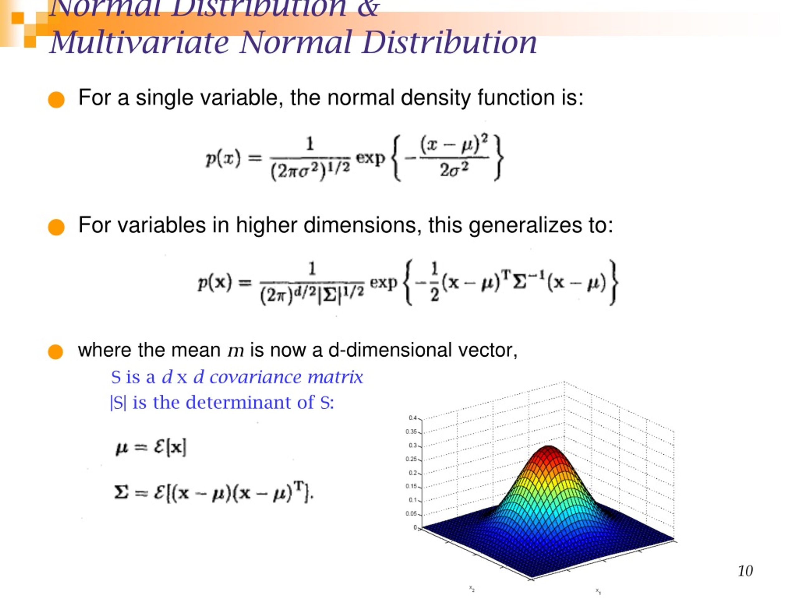
The Multivariate Normal (MVN) distribution is the natural extension of this idea to multiple dimensions, where we're modeling a vector of random variables. To do this, we simply upgrade our parameters from scalars to vectors and matrices:

• The mean becomes a mean vector $\vec{\mu }$, where each element is the mean of one variable. This vector defines the center of the distribution in a multi-dimensional space.
• The variance becomes a covariance matrix $\Sigma$, which we studied in the last lesson. This matrix defines both the spread (variance) of each variable and the correlation between them.

To formalize this and understand the notation, let's watch the beginning of the following video.

The Probability Density Function (PDF)

Just as the univariate normal has a specific formula for its bell curve, the MVN has a PDF that defines its "bell surface" in higher dimensions. The formula is:

$f(\mathbf{y})=\frac{1}{(2\pi {)}^{p/2}|\mathbf{\Sigma }{|}^{1/2}}\exp \left(-\frac{1}{2}(\mathbf{y}-\vec{\mu }{)}^{\prime }{\mathbf{\Sigma }}^{-1}(\mathbf{y}-\vec{\mu })\right)$

This might look intimidating, but it's a direct parallel to the univariate case. The term in the exponent, $(\mathbf{y}-\vec{\mu }{)}^{\prime }{\mathbf{\Sigma }}^{-1}(\mathbf{y}-\vec{\mu })$, is a matrix equivalent of the squared distance from the mean, scaled by the inverse of the covariance. This is what creates the elliptical or "bell" shape. This term is known as the Mahalanobis distance.

2. The Geometry of the Multivariate Normal Distribution

The true intuition for the MVN comes from understanding how the mean vector and covariance matrix define its shape.

• The Mean Vector $\vec{\mu }$: This is straightforward. It sets the center or peak of the distribution.
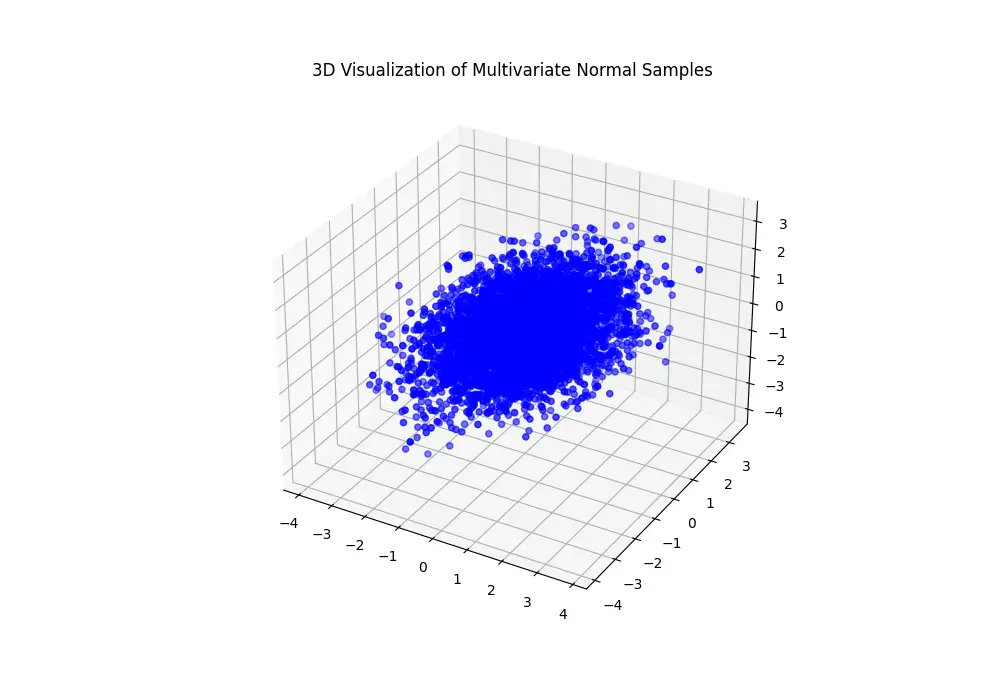
• The Covariance Matrix $\Sigma$: This is where the magic happens. It determines the spread, shape, and orientation of the data cloud.

Imagine slicing through the 3D bell shape at a certain height. The outline of that slice will be an ellipse. These outlines are called contours of constant probability. The shape of these ellipses is dictated entirely by $\Sigma$.

The following video provides an excellent geometric interpretation.

As the video explained, the connection between the covariance matrix and the geometry of the distribution is one of the most beautiful concepts in multivariate statistics. Your background in linear algebra will be very helpful here.

• The eigenvectors of $\Sigma$ give the directions of the principal axes of the ellipse.
• The eigenvalues of $\Sigma$ give the variance along those principal axes. The larger the eigenvalue, the more spread out the data is along the corresponding eigenvector.

3. Key Properties and Their Importance

What makes the MVN so useful in machine learning are its powerful and elegant mathematical properties. Understanding these helps explain why certain models work the way they do.

Let's explore some of these properties using the excellent distill.pub article and the bookdown.org chapter for reference.

Now let's dive into the properties.

Property 1: Marginal and Conditional Distributions are Normal

This is a profound property. It means that if you start with a set of variables that are jointly normal, any subset you look at will also be normal.

• Marginalization: If a vector $[{\mathbf{y}}_1,{\mathbf{y}}_2]$ is MVN, then the distribution of just ${\mathbf{y}}_1$ (ignoring ${\mathbf{y}}_2$) is also a (simpler) MVN. Visually, this is like projecting the high-dimensional bell shape onto a lower-dimensional axis.
• Conditioning: If you observe the value of a subset of variables (e.g., you know ${\mathbf{y}}_2=a$), the distribution of the remaining variables (${\mathbf{y}}_1$) is still MVN, but with an updated mean and a smaller covariance. Visually, this is like taking a slice through the high-dimensional bell shape. This property is the mathematical foundation of Bayesian inference with Gaussian models.

Property 2: Linear Transformations are Normal

If $\mathbf{y}$ is an MVN random vector and you apply a linear transformation to it (i.e., multiply by a matrix $\mathbf{A}$ and add a vector $\mathbf{c}$), the resulting vector $\mathbf{Ay}+\mathbf{c}$ is also MVN.

• Importance: This is crucial in many engineering and statistical models where one set of variables is a linear function of another. For example, if you model sensor noise as MVN and the system's dynamics are linear, you can precisely calculate the distribution of the system's state. It guarantees that normality is preserved through linear models. The bookdown.org resource, under section 25.1.4.1 Properties of the Multivariate Normal Distribution, provides the straightforward formulas for the new mean and covariance.

Property 3: Zero Correlation Implies Independence

In a previous lesson, we established that if two variables are independent, their covariance (and correlation) is zero. However, the reverse is generally not true... except for the MVN distribution.

For variables that are jointly normally distributed, zero correlation is a necessary and sufficient condition for independence.

• Importance: This is an enormous simplification. To check for independence between two normally distributed variables, you only need to check if their covariance is zero. This simplifies model structures and assumptions dramatically. For instance, if your covariance matrix is diagonal, you know that all your variables are mutually independent.

Let's hear a clear explanation of this and the linear transformation property.

Conclusion

This lesson completes your tour of the fundamental probability distributions for machine learning. The Multivariate Normal distribution is a powerful tool for modeling continuous data in multiple dimensions.

Key Takeaways:

• The MVN is a generalization of the normal distribution, defined by a mean vector $\vec{\mu }$ (its center) and a covariance matrix $\Sigma$ (its shape and orientation).
• The geometry of the MVN is an ellipsoid, whose principal axes are determined by the eigenvectors of $\Sigma$ and whose spread along those axes is determined by the eigenvalues.
• The MVN has powerful properties that make it mathematically tractable and useful for modeling:
  • Its marginal and conditional distributions are also normal.
  • It is closed under linear transformations.
  • For MVN variables, zero correlation implies independence, which is a significant simplification.
• It serves as a foundational building block for many ML algorithms, including Gaussian Mixture Models, Linear Discriminant Analysis, Kalman Filters, and Gaussian Processes.

Next Steps:

Having covered the key distributions, our next module, "Statistical Inference and Estimation," will focus on a critical question: How do we determine the parameters of these distributions (like $\mu$ and $\Sigma$) from a set of observed data? We will begin by distinguishing between population parameters and sample statistics, and then dive into our first formal estimation technique: the Method of Moments.