Hello! Welcome to your fourth lesson in the "Probability and Distributions for Modeling Data" module.
In our last lesson, we focused on discrete distributions (Bernoulli, Binomial, and Poisson), which are perfect for modeling counts of events or successes. Today, we shift our attention to continuous data—measurements that aren't restricted to integer counts but can take any value within a range.
This lesson directly addresses the learning outcome: Model continuous measurements and waiting times using Normal and Exponential distributions. We will explore the two most important continuous distributions in machine learning:
- The Normal (or Gaussian) Distribution: Used for modeling symmetric, bell-shaped data like sensor measurements, human height, or test scores.
- The Exponential Distribution: Used for modeling waiting times between events, such as the time until a component fails or the time between customer arrivals.
Understanding these distributions is crucial for your goal of mastering the 'why' behind machine learning models, as many algorithms either assume your data follows one of these patterns or use them in their internal workings.
1. The Normal (Gaussian) Distribution: Modeling Measurements
The Normal distribution is arguably the most famous and widely used distribution in all of statistics. It appears so frequently in nature and data science that it was named "normal." You'll see it used to describe everything from IQ scores to the errors made by a predictive model.
It's characterized by its symmetric, bell-shaped curve. To fully define any normal distribution, you only need two parameters:
- The mean (), which sets the center (the peak) of the bell.
- The standard deviation (), which controls the spread or width of the bell.
The following video from Socratica provides an excellent introduction with real-world examples.
Normal Distributions Explained – With Real-World Examples
This video will build your intuition for the Normal distribution, explaining its key properties and parameters.
Watch the video from the beginning to 03:35. Focus on how the same bell shape appears in different contexts and how the mean (\mu) and standard deviation (\sigma) control the location and shape of the curve.
The Empirical Rule (68-95-99.7)
One of the most practical properties of the Normal distribution is the empirical rule. It gives you a quick way to understand how your data is spread around the mean, using the standard deviation as a yardstick.
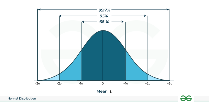
Specifically, for any Normal distribution:
- Approximately 68% of the data falls within 1 standard deviation of the mean ().
- Approximately 95% of the data falls within 2 standard deviations of the mean ().
- Approximately 99.7% of the data falls within 3 standard deviations of the mean ().
This rule is extremely useful for a quick sense-check of data and for identifying outliers. An observation more than 3 standard deviations away from the mean is very rare.
The next part of the Socratica video explains this rule with some great examples.
Normal Distributions Explained – With Real-World Examples
Now, let's see the empirical rule in action.
Watch the segment from 03:35 to 06:46. Pay attention to how the rule is applied to real data like head circumference. This gives you a concrete feel for what 'one standard deviation' means.
Calculating Probabilities with Continuous Distributions
In the last lesson, we used the Probability Mass Function (PMF) to find the probability of a specific count (e.g., exactly 3 successes). For continuous distributions, the concept is slightly different. We use a Probability Density Function (PDF).
The key idea is that for a continuous variable, the probability of it being exactly one specific value is zero. Think about it: what's the probability that a person's height is exactly 175.00000... cm? It's infinitesimally small.
Instead, we calculate the probability that a value falls within a range. This probability is represented by the area under the PDF curve for that range. You'll recall from your engineering studies that finding the area under a curve is done using integration. While the formula for the Normal PDF looks complex, you almost never have to do the integration by hand. In practice, we use software or a standardized approach.
The video below explains this concept and introduces a powerful tool for finding these probabilities: the z-score. A z-score tells you how many standard deviations a value is away from the mean, allowing you to compare values from different normal distributions.
Normal Distributions Explained – With Real-World Examples
This final segment from the Socratica video will clarify how probabilities are calculated and introduce the practical concepts of the PDF, CDF, and z-scores.
Watch from 10:43 to 15:15. Focus on the core ideas: Probability is the area under the curve. You don't need to integrate by hand; we use tools like the Cumulative Distribution Function (CDF), which gives the total area to the left of a point. A z-score standardizes your value, making it easy to look up probabilities using a standard normal table or software.
Many machine learning models, such as Linear Regression and Gaussian Naive Bayes, make assumptions that the data or the model's errors are normally distributed. As stated in the article "Understanding Normal Distribution in Machine Learning" (ID: LINK), ensuring these assumptions hold can improve a model's performance and interpretability.
2. The Exponential Distribution: Modeling Waiting Times
We now turn to our second key continuous distribution. Remember the Poisson distribution from our last lesson, which modeled the number of events in a fixed interval (e.g., 3 customers arrive per hour)? The Exponential distribution is its natural companion: it models the time between those events (e.g., the time until the next customer arrives).
The relationship is inverse:
- Poisson: How many events per unit of time?
- Exponential: How much time per event?
This video from zedstatistics provides a superb explanation of this connection and the distribution's core properties.
Exponential Distribution! AWESOME EXPLANATION. Why is it called "Exponential"?
This video clearly links the Exponential distribution back to the Poisson process, which we covered in the last lesson.
Watch from 00:50 to 07:56. Pay close attention to: The inverse relationship between Poisson and Exponential (e.g., cars per hour vs. hours per car). The key property of memorylessness. The relationship between the Poisson mean (\lambda, the event rate) and the Exponential mean (\mu = 1/\lambda, the average waiting time).
The "Memoryless" Property
Memorylessness is the defining characteristic of the Exponential distribution. It means that the probability of an event occurring in the next interval of time is independent of how much time has already passed. For example, if the average time between bus arrivals is 10 minutes and you've already been waiting for 5 minutes, the probability that the bus arrives in the next minute is the same as it was when you first got to the stop. The process "forgets" how long you've been waiting.
Calculating Probabilities with the Exponential Distribution
Unlike the Normal distribution's bell curve, the Exponential distribution's PDF is always decreasing. This means that shorter waiting times are more probable than longer ones.

To calculate the probability that the event happens within a certain time , we use its Cumulative Distribution Function (CDF):
Where is the rate parameter (the same from the corresponding Poisson process).
The zedstatistics video demonstrates how to use this formula to answer practical questions.
Exponential Distribution! AWESOME EXPLANATION. Why is it called "Exponential"?
Let's see how to apply the CDF formula to calculate probabilities for different waiting time scenarios.
Watch from 09:15 to 17:01. Focus on how to calculate the probability for three types of questions: The event occurs within a certain time (e.g., P(X < 10)). The event occurs after a certain time (e.g., P(X > 30)), which is calculated as 1 - P(X < 30). The event occurs at exactly a certain time, which is always 0 for a continuous distribution.
In machine learning, the Exponential distribution is fundamental to survival analysis, which models time-to-event data, such as how long a customer will remain subscribed or the lifespan of a mechanical part.
Test your understanding!
For each of the following scenarios, decide whether the Normal or Exponential distribution would be a better model and briefly explain why.
- A dataset contains the heights of all adult males in a large city.
- A call center wants to model the time between incoming phone calls. The average rate of calls is 60 per hour.
Show answer
- Normal Distribution. Human height is a classic example of a continuous measurement that tends to cluster around an average value, with fewer people at the very tall and very short extremes. The data would likely be symmetric and bell-shaped.
- Exponential Distribution. This scenario is about modeling the waiting time between events (phone calls) that occur at a known average rate. This is the exact use case for the Exponential distribution. The rate parameter would be calls/hour, or 1 call/minute.
Conclusion
You've now added two essential continuous distributions to your statistical toolkit. They provide the foundation for modeling a vast range of real-world phenomena and are critical assumptions in many ML algorithms.
Key Takeaways:
| Distribution | What It Models | Key Characteristics | Parameters |
|---|---|---|---|
| Normal | Continuous measurements that cluster around an average. | Symmetric, bell-shaped. | Mean () and Standard Deviation (). |
| Exponential | The waiting time between events in a Poisson process. | Decreasing curve, memoryless. | Rate (). The mean is . |
Next Steps:
You might be wondering why the Normal distribution is so common. It's not just a coincidence! In our next lesson, we will explore the Central Limit Theorem, a fundamental principle in statistics that explains why the Normal distribution emerges so frequently, especially when we work with averages of samples. This theorem is the theoretical backbone for much of statistical inference.