Interpreting Hierarchical Clustering and Dendrograms

1. What is Hierarchical Clustering?

Unlike k-means, which produces a single "flat" partitioning of the data for a given K, hierarchical clustering creates a multi-level structure of clusters. There are two main approaches:

• Agglomerative (Bottom-Up): This is the most common method. It starts by treating each data point as its own cluster and then progressively merges the two closest clusters until only one cluster (containing all points) remains.
• Divisive (Top-Down): This method starts with all data points in a single cluster and recursively splits them until each point is its own cluster.

We will focus on the agglomerative approach, as it's more widely used in practice.

The result of hierarchical clustering is a structure that is very intuitive to visualize. Let's look at an image that connects the raw data points to their clustered hierarchy.

2. The Agglomerative Clustering Process

The "bottom-up" logic of agglomerative clustering is straightforward. Let's walk through the steps conceptually.

1. Initialize: Start with each data point as a separate cluster.
2. Find Closest Pair: Identify the two clusters that are "closest" to each other based on a chosen distance measure.
3. Merge: Combine these two clusters into a new, single cluster.
4. Repeat: Repeat steps 2 and 3 until all data points have been merged into one large cluster.

To see this process in action, the following video provides an excellent visual explanation using a simple heatmap example.

This process naturally raises a critical question: what exactly do we mean by "closest"? Answering this involves two key choices: the distance metric and the linkage criterion.

3. Defining "Closest": Distance Metrics and Linkage Criteria

To implement the algorithm, we need to precisely define how we measure the distance between clusters.

Distance Metric: Measuring the Distance Between Points

First, we need a way to measure the distance between two individual data points. The most common choice is the Euclidean distance, which you can think of as the straight-line distance between two points. Given your engineering background, you'll recognize this as a direct application of the Pythagorean theorem, generalized to multiple dimensions.

Linkage Criterion: Measuring the Distance Between Clusters

Once we have clusters with more than one point, how do we measure the distance between them? This is determined by the linkage criterion. There are several methods, and the choice can significantly impact the final cluster structure. The most common ones are:

• Single Linkage: The distance between two clusters is the distance between the closest pair of points across the two clusters.
• Complete Linkage: The distance is determined by the farthest pair of points across the two clusters.
• Average Linkage: The distance is the average of all pairwise distances between points in the two clusters.
• Ward's Method: This method merges the pair of clusters that leads to the minimum increase in the total within-cluster variance. It tends to produce compact, similarly-sized clusters and is a very popular default choice.

The following video from StatQuest clearly explains both distance metrics and linkage criteria.

As you saw, your choice of distance and linkage is not trivial; it influences the shape and size of the clusters the algorithm identifies.

4. Interpreting the Dendrogram

The primary output of hierarchical clustering is the dendrogram. This tree diagram visualizes the entire merging process and is the key to interpreting the results.

How to Read a Dendrogram

• The leaves at the bottom are the individual data points.
• As you move up, horizontal lines indicate a merge.
• The vertical position (height) of the horizontal line indicates the distance (or dissimilarity) at which the two clusters were merged. Longer vertical lines mean that two clusters were merged at a greater distance, implying they are less similar.

The following video provides an excellent walkthrough of interpreting a dendrogram using a real-world example.

Choosing the Number of Clusters

As the video explained, one of the main advantages of hierarchical clustering is that you don't need to pre-specify the number of clusters. Instead, you can decide on the number of clusters after seeing the full hierarchy in the dendrogram. You do this by making a horizontal "cut" across the tree.

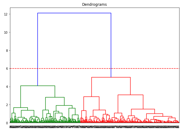
A common heuristic for deciding where to cut is to look for the longest vertical line that is not intersected by any horizontal merge lines. Cutting through this line often represents a good separation point because it corresponds to merging two very dissimilar groups.

The following reading explains this practical rule with clear illustrations.

Conclusion

Today you've learned a powerful and intuitive clustering method that complements k-means. Hierarchical clustering provides a rich, visual representation of your data's structure, freeing you from having to guess the number of clusters upfront.

Key Takeaways:

• Hierarchical Clustering builds a nested hierarchy of clusters, most commonly using an agglomerative (bottom-up) approach.
• The algorithm's behavior is defined by the distance metric (e.g., Euclidean) used for points and the linkage criterion (e.g., Ward's, Complete, Single) used for clusters.
• The dendrogram is a tree diagram that visualizes the entire merging process. The height of each merge represents the dissimilarity between the merged clusters.
• You can determine the final number of clusters by making a horizontal cut across the dendrogram. A good place to cut is often across the longest vertical line that doesn't cross a merge line.

Preview of the Next Lesson:

So far, both k-means and hierarchical clustering assign each data point to exactly one cluster (this is called "hard clustering"). But what if a data point could belong to multiple clusters with different probabilities? In our next lesson, we will explore Gaussian Mixture Models (GMMs), a probabilistic method that provides a "soft clustering" by calculating the likelihood that each point belongs to each cluster.