Optimal K-Means Clustering: Elbow Method & Silhouette Scores

1. The Elbow Method: Measuring Cluster Compactness

The first and most intuitive method for finding the optimal K is the Elbow Method. The core idea is to run the k-means algorithm for a range of K values and measure how "compact" the resulting clusters are for each K. We want clusters where the data points are packed tightly around their centroids.

The Metric: Within-Cluster Sum of Squares (WCSS)

To quantify compactness, we use a metric called the Within-Cluster Sum of Squares (WCSS). For a given set of clusters, WCSS is the sum of the squared distances of each data point to its assigned centroid. A smaller WCSS value means the clusters are denser.

In scikit-learn, this value is easily accessible as the inertia_ attribute of a fitted KMeans object. Your engineering background might find it helpful to think of WCSS as being analogous to the total variance within all clusters; minimizing WCSS is like minimizing this internal variance.

To understand the concept and calculation of WCSS more deeply, let's turn to a video.

Finding the "Elbow"

As the video explained, the process is as follows:

1. Run k-means for a range of K values (e.g., from 2 to 10).
2. For each K, calculate the total WCSS.
3. Plot the number of clusters (K) on the x-axis and the corresponding WCSS on the y-axis.

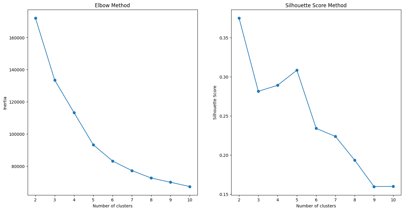
As you increase K, the WCSS will always decrease. This is because with more clusters, each cluster becomes smaller and tighter. If K equals the number of data points, WCSS would be zero, but this is useless as each point would be its own cluster. We are looking for a point of diminishing returns.

This point is called the "elbow"—it's the spot on the graph where the WCSS starts to decrease much more slowly.

Drawbacks of the Elbow Method

While intuitive, the Elbow Method has a significant practical limitation: the elbow is often not clear.

This ambiguity makes the method subjective and sometimes unreliable. This is why we need a more robust technique, which brings us to the Silhouette Method.

2. The Silhouette Method: A More Robust Approach

The Silhouette Method is generally preferred because it considers two criteria instead of one:

• Cohesion: How close are the data points within the same cluster? (Measured by average intra-cluster distance, a).
• Separation: How far apart are the data points from other clusters? (Measured by average nearest-cluster distance, b).

A good clustering has high cohesion (small a) and high separation (large b).

The Metric: Silhouette Score

The silhouette score for a single data point is calculated with the formula:
$S=\frac{b-a}{\max (a,b)}$

The score ranges from -1 to +1:

• +1: The point is well-clustered, far from other clusters.
• 0: The point is on or very close to the boundary between two clusters.
• -1: The point is likely assigned to the wrong cluster.

To find the best K, we typically calculate the average silhouette score for all data points for each value of K. The K that yields the highest average score is considered optimal.

To understand this concept more clearly, the following video explains the calculation and interpretation.

As the video shows, and in contrast to the elbow plot, we look for the peak (maximum value) in the silhouette score plot. Refer back to the right-hand plot in the "Elbow Method and Silhouette Score Method" image above—the highest score is at K=4.

A Deeper Look with Silhouette Plots

While the average score is a good indicator, a much more powerful diagnostic tool is the silhouette plot. This visualization shows the silhouette score of every single data point, grouped by cluster.

To summarize the key points from the article, when comparing silhouette plots for different K values, you are looking for:

1. Highest Average Score: The red dotted line should be as high as possible.
2. Uniform Thickness: The "blades" (the colored shapes representing each cluster) should be of similar thickness, indicating that clusters are of a balanced size.
3. Few Low Scores: Most points in a cluster should have scores above the average. Wide blades are good.
4. No Negative Scores: The presence of scores below zero indicates that points may have been misclassified.

Using these criteria provides a much richer and more reliable way to select K than just looking at the average score or a potentially ambiguous elbow.

Conclusion

You now have a powerful and practical toolkit for one of the most common questions in clustering. While data exploration and domain knowledge always play a role, these quantitative methods provide a strong, data-driven foundation for your modeling decisions.

Key Takeaways:

• Choosing the right number of clusters, K, is essential for meaningful results with the k-means algorithm.
• The Elbow Method uses WCSS (inertia) to find the "point of diminishing returns" in cluster compactness, but the result can be subjective and ambiguous.
• The Silhouette Method is more robust because it evaluates both cluster cohesion (a) and separation (b).
• You can select K by finding the peak in an average silhouette score plot or, for a more detailed analysis, by inspecting silhouette plots to find the K that produces clusters of uniform size and high scores.
• It is often wise to use both methods as a cross-check to build confidence in your choice of K.

Preview of the Next Lesson:

In this and the previous lesson, we've focused on a clustering method that requires us to specify the number of clusters beforehand. But what if we don't want to make that choice? In our next lesson, we will explore a different approach: Hierarchical Clustering, where we will build a tree of clusters and interpret the resulting structure using a dendrogram.