Introduction to Gaussian Mixture Models

1. From Hard to Soft Clustering: The Need for a Probabilistic Approach

Let's start by revisiting a core limitation of k-means. As we've seen, k-means works well for simple, well-separated, and roughly circular clusters. However, its rigid assumptions cause problems in many real-world scenarios.

To understand these limitations visually and see why a more flexible model is needed, please read the following section from the Python Data Science Handbook.

As you saw, k-means performs poorly on non-circular clusters and provides no measure of confidence for its assignments. Points on the boundary between two clusters are assigned to one or the other with 100% certainty, which is often unrealistic.

This is the distinction between hard clustering (k-means) and soft clustering (GMMs).

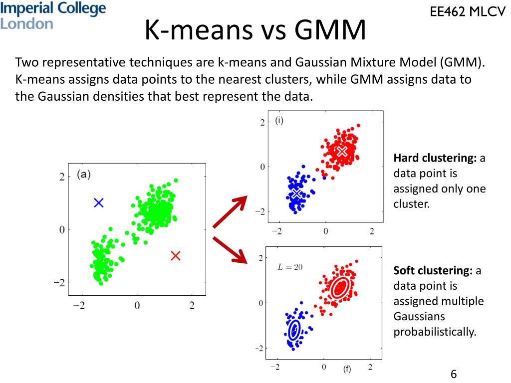
GMMs address both limitations of k-means:

1. They can adapt to elliptical cluster shapes.
2. They provide a probabilistic assignment, indicating the likelihood that a point belongs to each cluster.

2. What is a Gaussian Mixture Model?

A Gaussian Mixture Model approaches clustering by assuming that the data points are generated from a mixture of several Gaussian (or normal) distributions. Each of these Gaussian distributions represents a cluster.

Given your engineering background, you're familiar with the normal distribution as the classic "bell curve." A GMM is simply a combination of several of these, each with its own properties, that together form the overall distribution of the data.

Each Gaussian component in the mixture is defined by three key parameters:

• Mean ($\mu$): A vector representing the center of the cluster.
• Covariance ($\Sigma$): A matrix that describes the shape and orientation of the cluster. This is the crucial parameter that allows GMMs to model elliptical shapes, unlike the strict circular assumption in k-means.
• Mixing Probability (${\pi }_k$): The weight or size of the k-th Gaussian component. It represents the probability that a data point was generated from that cluster, with the sum of all mixing probabilities being 1.

The following video provides an excellent and intuitive introduction to these core concepts.

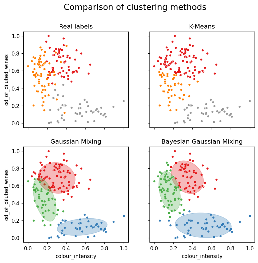
The ability to have a full covariance matrix for each cluster is what gives GMM its flexibility. In practice, when using libraries like Scikit-Learn, you can control the complexity of the cluster shapes through a hyperparameter, often called covariance_type. You can constrain the shapes to be spherical (like k-means), diagonal (ellipses aligned with the axes), or full (ellipses with any orientation).

3. How GMMs Learn: The Expectation-Maximization (EM) Algorithm

So, if our data is a mixture of Gaussians, how do we figure out the mean, covariance, and mixing weight for each of them? The answer is an iterative algorithm called Expectation-Maximization (EM).

The EM algorithm is conceptually similar to the iterative process in k-means but is more powerful. It finds the model parameters that maximize the likelihood of the observed data. It works by cycling between two steps:

1. E-Step (Expectation): This is the "soft assignment" step. Given the current parameters for each cluster (mean, covariance, weight), we calculate the probability that each data point belongs to each cluster. This probability is often called the point's responsibility for each cluster. A point lying midway between two cluster centers might have a 50% responsibility for each.

2. M-Step (Maximization): This is the "update" step. We re-calculate the parameters for each cluster. The new mean, covariance, and weight for a cluster are calculated as a weighted average over all data points, where the weights are the responsibilities computed in the E-step. Points that are more likely to belong to a cluster have more influence on its new parameters.

The algorithm repeats these E and M steps until the parameters stop changing significantly, meaning the model has converged.

The following video provides a fantastic explanation of the EM algorithm and, more importantly, a visual demonstration of it in action.

The visualization in the video is key. It shows how the algorithm starts with a rough guess and gradually "walks" the Gaussian components over the data until they find a good fit, perfectly illustrating the iterative nature of the EM algorithm.

Conclusion

Today, we've taken a significant step from hard clustering to the more nuanced world of probabilistic, or soft, clustering with Gaussian Mixture Models.

Key Takeaways:

• GMMs are a probabilistic clustering method that models data as a mixture of several Gaussian distributions.
• This approach overcomes key limitations of k-means by handling elliptical cluster shapes and providing soft (probabilistic) assignments.
• Each cluster (Gaussian component) is defined by its mean ($\mu$), covariance ($\Sigma$), and mixing weight ($\pi$).
• The Expectation-Maximization (EM) algorithm is used to find these parameters by iteratively performing two steps:
  • E-step: Calculate the probability ("responsibility") of each point belonging to each cluster.
  • M-step: Update the cluster parameters using a weighted average based on these responsibilities.

Preview of the Next Lesson:

We've introduced the EM algorithm and seen its intuition today. In the next lesson, we will formalize this understanding. Our learning outcome will be to explain the intuition of the Expectation-Maximization (EM) algorithm for fitting GMMs. We will take a closer look at the objective function that EM optimizes and understand why it's guaranteed to improve the model's fit to the data with every iteration.