Time-Series Data with Pandas

Part 1: Your Data's Home - The Pandas DataFrame

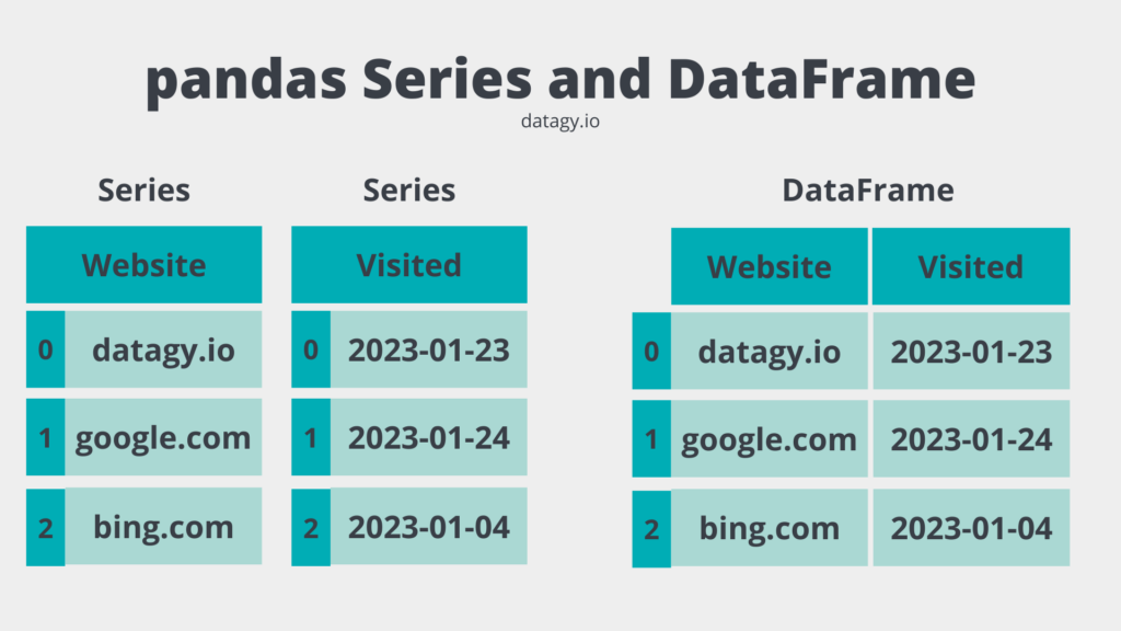
Think of a pandas DataFrame as a smart, programmable spreadsheet or a digital ledger. It organizes your data into a table of rows and columns. In the context of trading, each row typically represents a point in time (a single candle), and the columns represent the data for that candle: Open, High, Low, Close, and Volume.

Storing and Loading Data Locally

In the last lesson, you fetched data directly from an API. However, constantly re-downloading the same historical data is inefficient. A common workflow is to download the data once and save it to a local file, like a Comma-Separated Values (CSV) file.

Let's modify the script from our last lesson to save the data.

import yfinance as yf

# Fetch daily data for SPY for the year 2023
spy_data = yf.download(
    tickers="SPY",
    start="2023-01-01",
    end="2023-12-31",
    interval="1d",
    progress=False
)

# Save the DataFrame to a CSV file named 'spy_2023.csv'
# The index=True part ensures the Date index is saved in the file.
spy_data.to_csv('spy_2023.csv')

print("Data for SPY has been saved to spy_2023.csv")

Now, you have a file named spy_2023.csv in the same folder as your script. You can open it in a text editor or spreadsheet program to see the raw data.

To use this data in another script, you can load it directly from the file using pd.read_csv().

import pandas as pd

# Load the data from the CSV file
loaded_data = pd.read_csv('spy_2023.csv')

# Display the first 5 rows
print(loaded_data.head())

When you run this, you'll see the data you saved. But notice something important: the 'Date' column is just another column, and the index is a simple integer sequence (0, 1, 2...). This isn't ideal for time-series analysis. This brings us to our next, crucial topic.

Part 2: Making Time Work for You

For time-series analysis, the date and time information is not just another piece of data—it's the backbone of your entire dataset. Pandas needs to understand that your index represents moments in time. When loaded from a CSV, dates are often treated as simple text strings (which pandas calls object dtype). We need to convert them into datetime objects.

The following video from Corey Schafer provides an excellent, detailed explanation of how to work with time-series data in pandas. It uses cryptocurrency data, which is very similar to the forex and futures data you're interested in.

Let's apply these concepts to our loaded_data.

import pandas as pd

# Load the data from the CSV file
df = pd.read_csv('spy_2023.csv')

# --- Step 1: Convert the 'Date' column to datetime objects ---
# Pandas is smart and can often figure out the format automatically.
df['Date'] = pd.to_datetime(df['Date'])

# --- Step 2: Set the 'Date' column as the DataFrame's index ---
# The 'inplace=True' argument modifies the DataFrame directly.
df.set_index('Date', inplace=True)

# Let's inspect our DataFrame now
print("DataFrame Info:")
df.info()

print("\nFirst 5 rows with DatetimeIndex:")
print(df.head())

When you run df.info(), you'll now see that the index is a DatetimeIndex. This unlocks powerful new abilities. For example, you can select all the data from a specific month with remarkable ease:

# Select all data from January 2023
january_data = df.loc['2023-01']
print("\nData for January 2023:")
print(january_data)

# Select data for the first week of February 2023
first_week_feb = df.loc['2023-02-01':'2023-02-07']
print("\nData for the first week of February 2023:")
print(first_week_feb)

This intuitive slicing is impossible if your 'Date' column is just a string.

Part 3: Basic Data Manipulation

With a properly formatted DataFrame, you can now start to extract insights and prepare for analysis. This is similar to applying filters or creating new formula columns in a spreadsheet.

The article below gives a concise overview of these fundamental operations.

Let's try these operations:

# --- Selecting a Column ---
# This gives you a pandas Series of all the closing prices.
close_prices = df['Close']
print("\nClosing Prices:")
print(close_prices.head())

# --- Filtering Rows (Boolean Indexing) ---
# Find all days where the closing price was above $450.
high_close_days = df[df['Close'] > 450]
print("\nDays with Close > $450:")
print(high_close_days)

# --- Adding a New Column ---
# Let's calculate the daily candle range (High - Low), an important metric.
df['Range'] = df['High'] - df['Low']
print("\nDataFrame with 'Range' column:")
print(df.head())

# This filters the DataFrame to show only rows where the 'Range' column value is > 5.
big_range_days = df[df['Range'] > 5]
print(big_range_days)

Part 4: Programmatic Multi-Timeframe Analysis with Resampling

This is one of the most powerful time-series features in pandas and directly relates to your ICT analysis, which relies heavily on looking at market structure across different timeframes. Resampling is the process of changing the time frequency of your data.

You can downsample (e.g., convert 15-minute data into 1-hour data) or upsample (e.g., convert daily data into 12-hour data, though this is less common and requires filling in gaps).

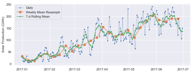
When you downsample OHLCV data, you need to tell pandas how to aggregate the candles. For example, to convert hourly data to daily data:

• The Open for the day is the open of the first hour.
• The High for the day is the maximum high of all hours.
• The Low for the day is the minimum low of all hours.
• The Close for the day is the close of the last hour.
• The Volume for the day is the sum of the volume from all hours.

The Corey Schafer video you watched earlier has an excellent section explaining resample(). Let's watch it again, this time focusing on the aggregation logic.

Now, let's apply this to our daily SPY data and resample it into weekly candles.

# Define the aggregation rules in a dictionary
ohlc_agg_rules = {
    'Open': 'first',  # The week's open is the 'first' open of the week
    'High': 'max',    # The week's high is the 'max' high of the week
    'Low': 'min',     # The week's low is the 'min' low of the week
    'Close': 'last',  # The week's close is the 'last' close of the week
    'Volume': 'sum'   # The week's volume is the 'sum' of daily volumes
}

# Resample the daily data ('D') to weekly data ('W')
weekly_df = df.resample('W').agg(ohlc_agg_rules)

# The 'W' frequency defaults to ending on Sunday. 
# We can also use 'W-FRI' to align with the trading week ending on Friday.
weekly_df_fri = df.resample('W-FRI').agg(ohlc_agg_rules)


print("Weekly Data (ending Sunday):")
print(weekly_df.head())

print("\nWeekly Data (ending Friday):")
print(weekly_df_fri.head())

Just like that, with a few lines of code, you have programmatically generated weekly candles from daily data. This is a fundamental building block for automating your multi-timeframe analysis.

Conclusion

You've made a huge leap forward today. You've gone from just downloading data to actively loading, storing, and manipulating it to suit your analytical needs.

Key Takeaways:

• A DataFrame is your primary tool for handling market data, like a programmable spreadsheet.
• Saving data to a CSV file is a standard practice to avoid repeated downloads.
• Converting date columns to a DatetimeIndex is essential for effective time-series analysis and enables intuitive slicing of data.
• You can easily select columns, filter rows based on conditions, and add new columns with calculated values.
• Resampling (.resample().agg()) is a powerful technique for programmatically changing timeframes, a cornerstone of multi-timeframe analysis in ICT.

Preview for the Next Lesson:
Real-world data is rarely perfect. Sometimes there are gaps (missing candles) due to holidays or data feed issues. In our next lesson, "Clean and preprocess raw market data to handle missing values," we will tackle this reality. You'll learn how to identify and handle these imperfections to ensure your analysis and future trading bot are running on robust, clean data.