Diagnosing Median Latency Regressions

The Puzzle: A Rising Median with a Stable Tail

Let's start by framing the scenario. A change in latency where p50 increases while p99 stays flat is often a sign of a shift in the entire distribution, rather than the "tail-widening" we associate with queueing or contention.

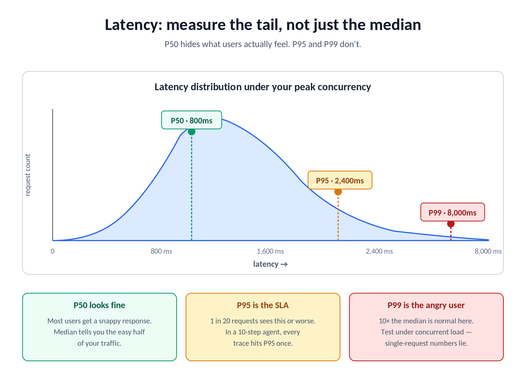
When the tail of the distribution stretches (e.g., p99 jumps while p50 is stable), it often points to a subset of requests hitting a bottleneck—like waiting for a database lock or a full connection pool. But when the median shifts without affecting the extreme tail, it suggests something more fundamental has changed about the work being done.

This is a critical distinction that guides your entire investigation. The following resource provides an excellent overview of these distribution shapes.

With this model in mind—a "whole distribution shift"—the question is no longer "What's causing a few requests to be slow?" but rather "Why has the work for the typical request changed?" Let's walk through a checklist of common culprits.

The Diagnostic Checklist

A senior engineer's value lies in methodical investigation, not guesswork. When faced with this p50 regression, you must resist the urge to immediately blame a database or a downstream service. The root cause is often more subtle and relates to how the data is being generated and aggregated.

The following checklist provides a structured approach.

Let's break down these checks in more detail.

1. Check the Traffic Mix (Simpson's Paradox in Action)

This is the most frequent cause of a median-only regression. The overall performance of your service is a blend of the performance of all its individual endpoints or transaction types. If the proportion of fast and slow requests changes, the overall median will shift, even if the performance of each individual endpoint has not changed at all.

Consider a service with two endpoints:

• GET /items/{id} (fast cache lookup): 50ms
• POST /orders (slow DB write): 500ms

Scenario A (Before):

• Traffic is 90% GET /items and 10% POST /orders.
• Most requests are fast. The overall p50 will be very close to 50ms.
• The p99 will be determined by the slow POST /orders requests, around 500ms.

Scenario B (After):

• A new feature launch causes a surge in orders. The traffic is now 50% GET /items and 50% POST /orders.
• The performance of each endpoint is still 50ms and 500ms, respectively. No code is slower!
• However, with half the requests now being slow, the overall median (p50) will jump significantly, perhaps to around 275ms.
• The p99 remains anchored by the performance of the slowest endpoint, still around 500ms.

This statistical illusion, a form of Simpson's Paradox, is why your first step must always be to question the composition of the workload.

2. Check Labels and Aggregation ("Segment First")

The traffic mix problem is fundamentally an aggregation problem. You are being misled because you are looking at a single, aggregated metric for the entire service. The solution is to segment the data using labels.

Since you work with Prometheus and Grafana, you're already familiar with the power of labels (endpoint, verb, client_id, region, etc.). When you see a regression, your first instinct should be to break down the metric by its most important labels.

• Is the p50 regression visible across all endpoints, or just one?
• Does it affect all tenants, or is it isolated to a single large customer?
• Is it happening in all regions or just one?

This principle is so important it's worth making it a rule.

In the video below, the presenter briefly discusses a similar idea of "splitting" metrics to find the source of an issue.

3. Check the Time Windows

This is a simpler but equally common error. Are you comparing apples to apples? A performance comparison is only valid if the context is as similar as possible. Comparing your service's performance at 2 PM on a Tuesday (peak traffic) with its performance at 3 AM on a Sunday (off-peak) is meaningless. The workload volume, traffic mix, and system state (e.g., cache warmth) will be completely different.

Always ensure your comparison windows are equivalent:

• Same time of day.
• Same day of the week.
• Before and after a specific deployment or configuration change.

A Practical Diagnostic Workflow

Let's synthesize this into a step-by-step process you can apply the next time you see this pattern.

1. Challenge the Metric: See a p50 regression on a dashboard. Don't accept it at face value.
2. Verify the Time Window: Confirm the "before" and "after" periods are comparable (e.g., Tuesday 10-11 AM vs. Wednesday 10-11 AM).
3. Segment by Key Labels: Break down the latency metric by the most critical label, usually the API endpoint or transaction name.
   • sum(rate(http_server_requests_seconds_bucket[5m])) by (le, endpoint)
4. Analyze the Segments: Examine the p50 for each individual endpoint.
   • Hypothesis A: You find that the p50 of one or more individual endpoints has increased. This is a "whole distribution shift" and indicates that endpoint is now doing more work. Your investigation should now focus on that endpoint.
   • Hypothesis B: You find that the p50 for every individual endpoint is stable.
5. Check the Traffic Mix: If you confirmed Hypothesis B, the cause must be a shift in composition. Check the throughput (request rate) for each endpoint in the "before" and "after" windows. You will likely find that the proportion of traffic to your slower endpoints has increased.

You have now moved from a vague "latency is up" to a precise, evidence-based conclusion: "Overall p50 latency increased because of a 30% increase in traffic to the /orders endpoint, not because any part of the system became slower."

Conclusion

Diagnosing a median-latency regression when the tail remains stable is a fantastic test of a performance engineer's analytical discipline. It requires you to think like a statistician before you think like a systems engineer, questioning the data's composition before diving into code and infrastructure.

Key Takeaways:

• A rise in median (p50) latency without a corresponding rise in tail (p99) latency is often caused by a shift in the traffic mix, not a degradation in component performance.
• This is a form of Simpson's Paradox, where an aggregated metric can be misleading.
• Your primary diagnostic tool is segmentation. Always break down aggregated metrics by key labels like endpoint, region, or tenant.
• Follow a systematic checklist: confirm the signal by checking the time window, the traffic mix, and the aggregation method before forming a hypothesis about the root cause.

In our next lesson, we will introduce a foundational principle of systems performance: Little's Law. You will learn how to calculate and apply the relationship between throughput, concurrency, and response time, giving you another powerful tool for reasoning about system behavior and bottlenecks.