Applying Little's Law to Performance Metrics

The Foundation: Little's Law

At its heart, Little's Law describes the relationship between the number of items in a system, how long they stay, and the rate at which they move through. Its elegance lies in its simplicity and universality.

The following resource provides a crisp introduction to the formula and its variables, translating them from their academic origins in queuing theory into terms you use every day in the context of distributed systems.

As you've just read, the law is stated as:

$L=\lambda \times W$

Where, for our purposes as performance engineers:

• L is Concurrency: The average number of requests being processed simultaneously in the system (sometimes called "in-flight" or "active" requests).
• λ (lambda) is Throughput: The average rate at which requests arrive (and, in a stable system, depart), measured in requests per second.
• W is Latency: The average time a request spends in the system, from start to finish, measured in seconds.

So, for us, the formula becomes:

Concurrency = Throughput × Latency

If you know any two of these values, you can calculate the third. For example, if a service is handling 200 requests per second (throughput) and each request takes an average of 0.5 seconds (latency), the average number of concurrent requests is:

$\text{Concurrency}=200\text{ req/s}\times 0.5\text{ s}=100\text{ requests}$

This means that, on average, there are 100 requests active in the system at any given moment.

Why This Matters: From Formula to Insight

Knowing the formula is one thing; applying it to gain insight is what separates a junior from a senior engineer. Little's Law is a powerful tool for resource planning, result validation, and bottleneck diagnosis.

The Latency Effect: Quantifying the Cost of Slowness

Little's Law makes it startlingly clear how latency impacts resource requirements. A slower system needs more concurrent capacity to sustain the same throughput, consuming more memory, threads, and connections.

The chart below provides a stark visualization. To achieve the same throughput of 200 req/sec, a system with 2-second latency requires four times the concurrency (and thus, resources) as a system with 0.5-second latency.

This chart illustrates Little's Law by comparing a "Fast System" (0.5s latency) and a "Slow System" (2s latency). To maintain an identical throughput of 200 req/sec, the slow system must handle 400 concurrent requests, four times the 100 requests handled by the fast system.

This isn't just about user experience; it's about cost and efficiency. A 10% latency improvement can translate directly into a 10% reduction in the concurrent resources needed, which can be a significant saving in a large-scale cloud environment.

The following reading expands on this and other practical applications, such as capacity planning and identifying bottlenecks.

Application in Your World: Workload Modeling

Your experience with JMeter involves setting a number of "concurrent users" (threads) and having them execute a script. Little's Law is the theoretical basis for calculating how many users you need to generate a specific target throughput. However, in this context, we must use a variation of the law that accounts for user "think time" and script pacing.

The formula for this closed-loop model is:

Number of Users = Throughput × (Response Time + Think Time + Pacing)

Let's watch a short video that explains this application in the context of performance testing.

This is an incredibly practical application. For example, if an architect provides a non-functional requirement of "3600 transactions per hour," you can use Little's Law to translate that into a concrete test configuration.

The following resource gives a great example of using this formula not just for planning, but for validating test results.

Knowing the Limits: When the Law "Breaks"

Little's Law is powerful, but it has one major prerequisite: it applies to stable systems in a steady state. A steady state is a condition where, on average, the rate of arrivals equals the rate of departures. The number of requests in the system might fluctuate, but it revolves around a stable average.

What happens when the arrival rate exceeds the system's capacity to process requests? The system is no longer stable. The queue of waiting requests grows, and latency increases without bound. This is often called thrashing.

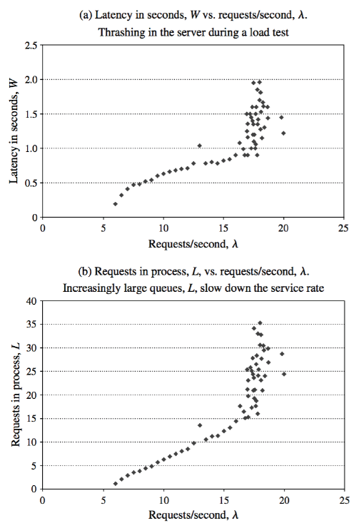
These plots show data from a real server load test. As requests per second (λ) increase, latency (W) and requests in process (L) remain stable at first. However, beyond a certain point (~15 req/s), the system saturates, and both latency and the number of queued requests increase dramatically. This is the point where the "steady state" assumption of Little's Law breaks down.

This transition from a stable state to a saturated one is a key behavior you look for in load tests. We will explore this "saturation knee" in detail in a future module on scalability analysis.

Finally, a crucial caveat: Little's Law operates on averages. Your last lesson was all about why averages can be deceiving and why percentiles (p95, p99) are so important. The concurrency calculated by Little's Law is an average concurrency. Due to natural variation, the peak concurrency will be higher. Always keep this in mind.

Conclusion

You have now added one of the most fundamental principles of performance engineering to your toolkit. Little's Law provides an essential framework for reasoning about system behavior under load.

Key Takeaways:

• Little's Law provides a simple formula connecting three key metrics: Concurrency = Throughput × Latency.
• It is not just a formula; it's a tool for resource sizing, capacity planning, and validating test results.
• Higher latency directly increases the concurrency required to sustain a given throughput, impacting resource consumption and cost.
• For closed-loop load testing (like with JMeter), you must use the variant that includes think time and pacing.
• The law's primary limitation is that it applies only to stable systems in a steady state and operates on averages, which can hide important tail-latency behavior.

In our next lesson, we will build directly on this foundation by learning how to formally identify the steady-state period in a load test, distinguishing it from warm-up and cool-down phases. This is the exact period where Little's Law holds true and where your most important measurements are taken.