Welcome back! In our last lesson, we delved into Little's Law, establishing the fundamental relationship between concurrency, throughput, and latency. A key insight was that this law, and indeed most meaningful performance analysis, applies to systems in a steady state. This naturally leads to a crucial question: how do we identify this "steady state" in the messy reality of a load test?
Today, we will answer that question. This lesson focuses on the lifecycle of a controlled load test and how to properly separate the data into three distinct phases: warm-up, steady-state, and cool-down. Mastering this skill is non-negotiable for a senior performance engineer. It is the bedrock of reliable analysis, ensuring that your conclusions about system performance are based on valid, representative data, not on the noisy and misleading artifacts of a system that is still starting up.
The Three Phases of a Well-Designed Load Test
A common mistake in performance testing is to treat the entire test run as a single block of data. This approach invariably leads to incorrect and indefensible results. A professionally executed test is understood as a process with distinct phases, each with its own purpose.
The following article from Octocore Performance provides an excellent breakdown of these phases and the technical reasons for their existence.
Warm-up and Steady State: the phases of a performance test | Octocore Performance
This article clearly defines the phases of a performance test and explains the underlying technical drivers for the warm-up period.
Please read the sections titled "Test Phases" and "Why Warm-up Matters". As you read, focus on how the technical events during warm-up (JIT compilation, cache filling, connection pool establishment) directly relate to the environment you work in with Java-based microservices, MySQL, and various caching layers.
As you've just read, the initial period of a test is not representative of normal operation. For the JVM-based applications you work with, the first few minutes involve intense activity that doesn't occur during normal, sustained operation:
- JIT Compilation: The JVM's C1 and C2 compilers are identifying "hot" methods and compiling them into highly optimized native code. This compilation consumes CPU and can cause initial requests to be significantly slower.
- Cache Priming: Your system's various caches—from Hazelcast distributed caches and application-level caches to the Cloud SQL buffer pool—are cold and empty. Initial requests will have high miss rates, leading to expensive trips to backend storage.
- Pool Initialization: Connection pools to your MySQL database and message queues like RabbitMQ are being established. The initial cost of creating these connections and performing handshakes is high.
Ignoring these initial effects and lumping them into your final analysis is a critical error.
Visualizing the Phases: From Plan to Reality
To manage these phases, you design a specific load profile in your test plan. A tool you're likely familiar with, the JMeter Ultimate Thread Group, provides a great way to visualize this plan.

This graph shows the intended load. The ramp-up period serves to gradually apply pressure and allow the system to warm up. The flat plateau is the intended steady state, the period where you want to measure performance. The ramp-down, or cool-down, allows you to observe how the system recovers.
Now, let's look at what the system's response might look like in a monitoring tool like Grafana.
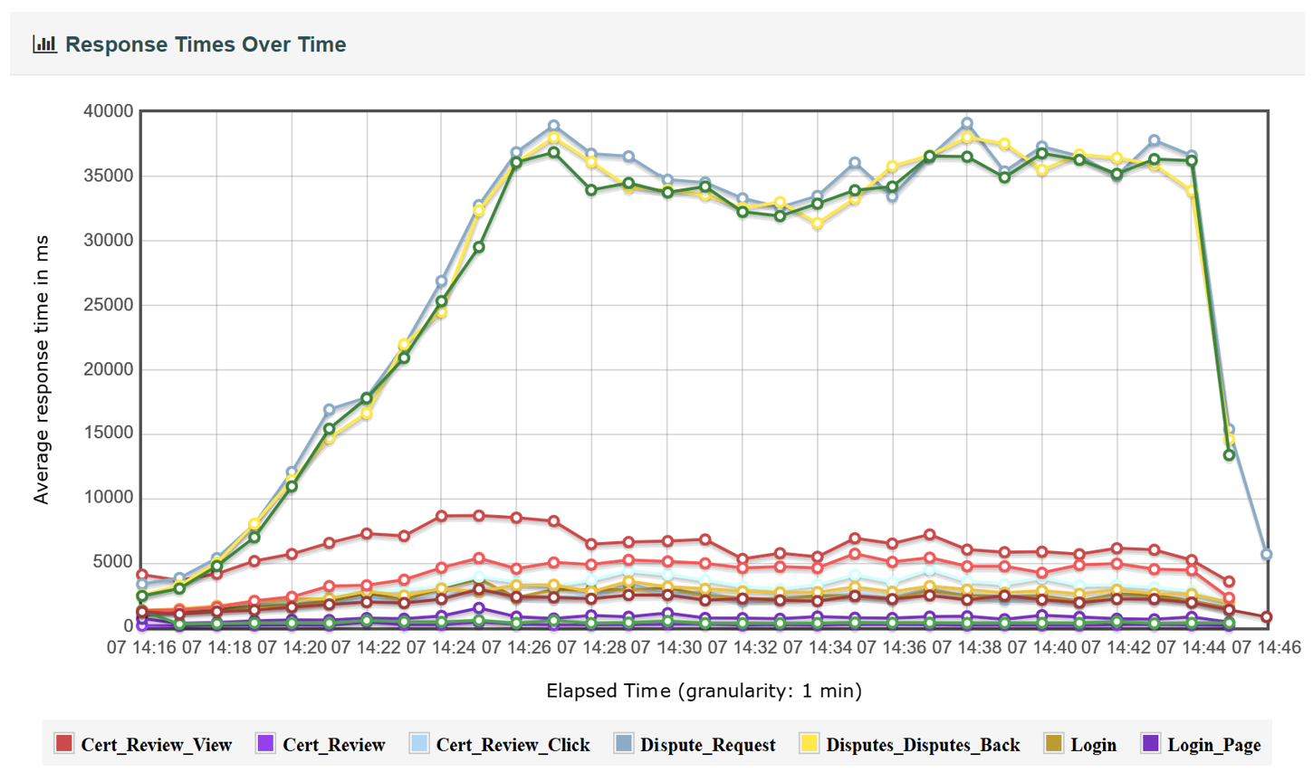
When you compare the two images, the relationship becomes clear:
- Warm-up: The rising line in the JMeter plan corresponds to the initial, volatile period in the response time graph (roughly from 07:14 to 07:26 in the chart). Response times are high and unstable as JIT compilation occurs, caches are populated, and connection pools are filled.
- Steady State: The flat plateau in the JMeter plan corresponds to the period where the response times stabilize (roughly 07:28 to 07:44). This is your measurement window. All your pass/fail criteria, SLO comparisons, and percentile calculations should be based exclusively on data from this period.
- Cool-down: The falling line in the JMeter plan corresponds to the sharp drop in response times at the end of the test (after 07:44) as load is removed.
The Consequences of Incorrect Analysis
Failing to isolate the steady state leads to contaminated metrics and invalid conclusions. The following resource reinforces why this separation is not just good practice, but a requirement for generating trustworthy results.
How to Conduct a Load Test in 7 Steps (2026 Playbook)
This article provides a practical checklist for load testing, with a strong emphasis on the validation and analysis steps.
Please read the subsection "Warm-Up, Steady State, and Cool-Down", and then in the section "Step 5 — Execute, Monitor, and Analyze", focus on the first point under the analysis framework. Pay close attention to the explicit instruction regarding SLA evaluation.
As the article states, including warm-up data inflates your p95 and p99 metrics. A test that might have actually passed its SLOs could be incorrectly failed because of a few slow initial requests. Conversely, if a code change introduces a subtle performance degradation, its effect could be lost in the noise of the warm-up period, leading you to incorrectly approve a problematic release. A senior engineer must be able to defend their results, and that defense starts with proving that the analysis was performed on a valid steady-state window.
Identifying Steady State in Practice
So, how do you determine precisely when the steady state begins?
- Visual Inspection (The Eyeball Method): As we did with the graph above, you look for the point where key metrics like response time, throughput, and error rates stabilize and form a relatively flat plateau. This is the most common and often sufficient method.
- Statistical Methods: For more rigor, you can apply statistical techniques. For example, you could calculate the standard deviation of response times within a moving time window (e.g., 1 minute). When that standard deviation drops below a certain threshold (e.g., 10% of the mean), you can declare the system to be in a steady state. This is an advanced technique that can be useful for automating analysis.
- Heuristics and Experience: Over time, you'll develop a feel for your systems. A stateless Go microservice might warm up in seconds. A large, monolithic Java application might need 5-10 minutes. Your experience with your specific stack (Spring Boot, Hazelcast, Cloud SQL) is your best guide, but it must always be confirmed by looking at the data.
Your primary action is to configure your analysis tools—whether it's a Grafana dashboard, a JMeter Listener, or a Python script—to ignore the initial N minutes of the test run, where N is the duration you've determined to be the warm-up period.
Conclusion
You now have a clear framework for structuring a load test and analyzing its results correctly. This is a foundational skill that separates amateur testing from professional performance engineering.
Key Takeaways:
- Every load test consists of three phases: warm-up, steady-state, and cool-down.
- The warm-up period is characterized by system initialization activities like JIT compilation and cache priming, resulting in unrepresentative performance metrics.
- The steady-state is the stable period where the system is operating under a consistent load. This is the only valid window for performance measurement and SLA evaluation.
- The cool-down period is for observing system recovery.
- You must actively exclude warm-up data from your analysis to avoid contaminated metrics (e.g., inflated percentiles) and incorrect conclusions.
- Identifying the start of the steady state can be done by visually inspecting graphs for stabilization or by using statistical methods.
Now that you know how to isolate a clean, reliable dataset from the steady-state period of a test, the next logical step is to analyze that data with statistical rigor. In our next lesson, we will explore how to determine whether an observed change in performance during the steady state is a real, practically meaningful regression or simply random noise in the system.