Calculating and Validating Latency Percentiles

Beyond the Average: Why a Single Number Lies

Imagine your team reports that the average response time for a critical API is 200ms. This sounds acceptable. However, this average could be hiding a serious problem. What if 95% of users get a snappy 50ms response, but the slowest 5% experience a frustrating 5-second wait? The average smooths over this terrible experience. Users don't experience the average; they experience their own specific response time. Focusing only on the average makes you blind to the users who are suffering the most.

To get a true picture of performance, we use percentiles. A percentile answers the question: "What was the experience for X% of my users?"

• p50 (Median): The 50th percentile. 50% of requests were faster than this value. This represents the typical experience.
• p95: The 95th percentile. 95% of requests were faster than this value. This is often considered the "worst-case" experience for the vast majority of users.
• p99: The 99th percentile. 99% of requests were faster than this value. This is often called "tail latency" and highlights the experience of the unluckiest 1% of requests.

This first resource provides a clear explanation of why percentiles are far more informative than averages.

The Calculation: From Raw Data to Insight

Now for the core of today's lesson: how do you actually compute these values? The process is straightforward and relies on one key operation: sorting.

Let's say you have a list of response times from a JMeter test run.

1. Collect the Data: Gather all the individual response time measurements into a single list.
2. Sort the Data: Arrange the list of response times in ascending order, from fastest to slowest.
3. Find the Index: Calculate the position (index) in the sorted list that corresponds to your desired percentile. For a list of N items and a percentile P (e.g., 0.95 for p95), the index is calculated as index = P * N. Since list indices are often 0-based in programming, you'll typically take the integer part of this result.
4. Find the Value: The latency value at that calculated index is your percentile.

Let's visualize this. Imagine you ordered 100 pizzas and tracked their delivery times. To find the p99 delivery time, you'd sort all 100 times from fastest to slowest and pick the 99th one in the list. The time for that pizza is your p99 latency.

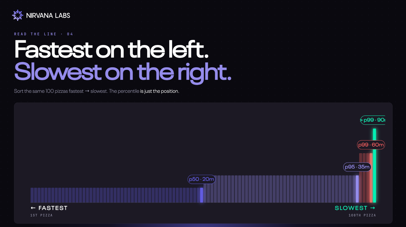
To see this calculation in action, let's watch a video that walks through the process with a simple dataset.

The logic is identical for any percentile. For a list of 10,000 latencies:

• p50 (Median): The value at index 0.50 * 10000 = 5000.
• p95: The value at index 0.95 * 10000 = 9500.
• p99: The value at index 0.99 * 10000 = 9900.

Verifying the Ordering: A Critical Sanity Check

Because percentiles are derived from a single sorted list of data, they have a natural and inviolable order. For any given dataset, it must always be true that:

This might seem obvious, but it's a powerful sanity check. If you write a script to parse a results file and it reports that p95 is less than p50, you have a bug in your calculation. There is no performance scenario where this ordering is not true.

The difference between these values is also highly informative.

• A small gap between p50 and p99 indicates consistent performance. Most users have an experience very similar to the typical user.
• A large gap between p50 and p99 indicates a long-tail latency distribution. While the typical experience might be good (low p50), a small fraction of users experience significantly worse performance.

This long-tail distribution is common in complex microservice systems and is often where the most challenging performance bottlenecks hide.

A Practical Python Implementation

Since you work with Python, let's look at how you'd implement this in code. It's a common task when building custom test harnesses or analysis scripts. The following resource contains a practical Python function for benchmarking Redis, but the latency calculation logic is universal.

Here is a standalone Python snippet based on that example. You can run this yourself to solidify your understanding.

# A sample list of 20 response times (in milliseconds)
latencies = [
    102, 78, 85, 91, 120, 
    88, 95, 105, 75, 82, 
    150, 93, 89, 250, 99, 
    110, 80, 450, 96, 101
]




# 1. Sort the list in ascending order
latencies.sort()




# The total number of measurements
n = len(latencies)




# 2. Calculate indices
p50_index = int(n * 0.50)
p95_index = int(n * 0.95)
p99_index = int(n * 0.99) # For small N, this might be the last element




# 3. Get the values at those indices
p50_latency = latencies[p50_index]
p95_latency = latencies[p95_index]
p99_latency = latencies[p99_index]

print(f"Sorted latencies: {latencies}")
print(f"Total measurements: {n}")
print("-" * 20)
print(f"P50 (Median) latency: {p50_latency} ms")
print(f"P95 latency: {p95_latency} ms")
print(f"P99 latency: {p99_latency} ms")




# 4. Verify the ordering
assert p50_latency <= p95_latency <= p99_latency
print("\nVerification successful: p50 <= p95 <= p99")

When you run this code, you'll see the sorted list and the calculated percentiles, which clearly follow the p50 <= p95 <= p99 rule.

Conclusion

Today we've moved beyond the simple average and embraced percentile-based latency analysis. This is a fundamental skill for any senior performance engineer, allowing you to understand the full range of user experience and to set meaningful performance targets.

Key Takeaways:

• Averages can hide significant performance problems; percentiles reveal the distribution of user experiences.
• The p50 (median) shows the typical experience, while p95 and p99 show the "tail latency" experienced by a minority of users.
• Calculating percentiles involves a simple three-step process: collect all measurements, sort them, and find the value at the index corresponding to the percentile.
• A critical sanity check is to verify the natural order: p50 <= p95 <= p99. If this is not true, your calculation is flawed.
• The gap between percentiles tells you about the consistency of your system's performance.

In our next lesson, we will apply this knowledge to a common diagnostic challenge: Diagnose a median-latency regression when tail latency appears unchanged. You'll see how understanding the difference between p50 and the tail is crucial for finding the root cause of subtle performance changes.