Key Performance Metrics in System Analysis

The Big Picture: How Fast vs. How Much

At the highest level, performance engineering is a balancing act between two primary concerns:

1. Latency: How fast is the system for a single user or request?
2. Throughput: How much work can the system handle in total?

These two are often in tension. A system optimized to handle a massive volume of requests might introduce small delays for each individual request. Conversely, a system tuned for the absolute fastest individual response might not scale to handle high traffic.

To get a quick overview of this fundamental trade-off, please watch the following short video.

Deconstructing Request Time

Now, let's break down what happens during the lifecycle of a single request. The term "response time" can be ambiguous, so we need to be more precise. We will distinguish between what the client experiences and what the server is actually doing.

• Response Time: From a user's or client's perspective, this is the total wall-clock time from the moment they send a request until they have received the entire response. This is often called "end-to-end time" and is what a tool like JMeter typically reports.
• Service Time: This is the time the server spends actively processing the request. It's the duration of productive work, such as executing code, running database queries, or computing a result.
• Wait Time (or Queue Time): This is the time a request spends idle on the server, waiting for a resource to become available before its service time can even begin. It might be waiting for a free worker thread, a database connection from a pool, or an available CPU core.

The relationship is simple but critical:

This server-side time is a major component of the end-to-end response time seen by the client. The following diagram illustrates this decomposition clearly.

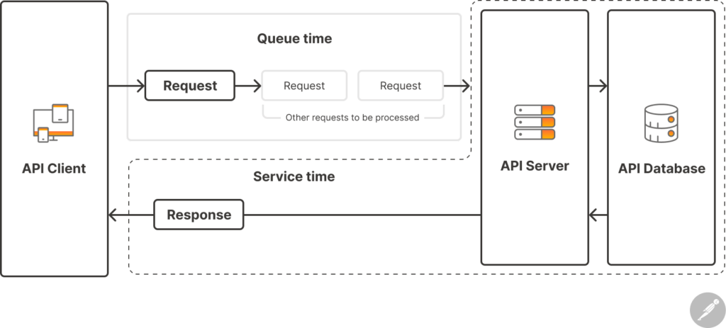
To explore this distinction further, let's watch a video that breaks down these components from a network perspective.

To solidify these definitions, let's turn to some written resources. The first article approaches these concepts from the perspective of queuing theory, which provides the mathematical foundation for performance analysis.

The Origin of Waiting: Utilization and Queuing

Why does "wait time" even exist? If a system has capacity, shouldn't it just process requests immediately? The answer lies in two factors: utilization and variability.

Utilization ($\rho$) is the proportion of time that a resource (like a CPU, a disk, or a service instance) is busy doing work. It's a ratio:
$\rho =\frac{\text{Demand}}{\text{Capacity}}=\frac{\text{Arrival Rate}}{\text{Service Rate}}$
For example, if requests arrive at a rate of 80 per second ($\lambda =80$), and the server can process 100 per second at full capacity ($\mu =100$), then the utilization is $\rho =80/100=0.8$, or 80%.

You might think that as long as utilization is below 100%, everything is fine. However, requests don't arrive in a perfectly uniform stream, and service times aren't always identical. This randomness means that sometimes, by chance, several requests will arrive in quick succession, forcing later ones to wait in a queue even if the server is, on average, not fully utilized.

As utilization gets higher, the probability of a new request arriving while the server is already busy increases. The queue gets longer, and the wait time grows—not linearly, but exponentially.

This graph is one of the most important visuals in performance engineering. It demonstrates why running systems "hot" (e.g., at 95% CPU utilization) is often a recipe for poor latency. A small increase in load can cause a massive increase in response time.

Let's read a bit more about utilization and its effect on queuing.

The Unifying Law: Throughput and Concurrency

We've covered the time-based metrics. Now let's formally define the rate- and count-based ones.

• Throughput (X): The rate at which requests are successfully completed over a period. It's measured in requests per second (RPS), transactions per second (TPS), or similar units. In your Prometheus queries, this is what you measure with functions like rate() or increase().
• Concurrency (N): The number of requests being handled by the system at the same time. These are the "in-flight" requests, which could be in a state of being actively served or waiting in a queue.

These three metrics—Response Time, Throughput, and Concurrency—are elegantly linked by a fundamental principle of systems theory called Little's Law.

Or, in our terms:

This law is incredibly powerful. It holds for any stable system and allows you to sanity-check your measurements. For example, if your load test tool reports a throughput of 200 TPS and an average response time of 500ms (0.5s), you can calculate the average number of concurrent requests in the system:

Concurrency = 200 TPS × 0.5 s = 100 requests.

If your APM tool shows a vastly different number of in-flight requests, it signals a potential measurement problem or a misunderstanding of the system's boundaries.

Let's read a final excerpt that ties these concepts together from a practical testing point of view.

Tying It All Together: A Scenario

Let's apply these concepts to a scenario using your toolchain. Imagine you're analyzing a performance test for a checkout microservice:

• JMeter reports:
  • Average Response Time: 1,800ms
  • Throughput: 100 TPS
• Pinpoint APM trace for the checkout service shows an average transaction duration of 1,500ms, broken down as:
  • 1200ms waiting for a connection from the Cloud SQL database connection pool.
  • 300ms of active processing (validating the cart, calculating totals, and running a DB insert).
• Prometheus/Grafana dashboards show:
  • Checkout service pods: CPU Utilization at 25%.
  • Cloud SQL (MySQL) instance: CPU Utilization at 98%.

How would you apply our vocabulary here?

• Response Time: 1,800ms (the full end-to-end time measured by the client, JMeter). The 300ms difference between this and the APM time (1,500ms) is likely network latency between JMeter and the service.
• Wait Time: 1,200ms. This is the time the request was queued inside the checkout service, waiting for a database connection.
• Service Time: 300ms. This is the time the checkout service was actively working.
• Utilization: 25% for the service, 98% for the database.
• Throughput: 100 TPS.
• Concurrency (within the checkout service, via Little's Law): $100\text{ TPS}\times 1.5\text{ s}=150$ concurrent requests.

The diagnosis is clear: the checkout service itself is not the bottleneck (only 25% CPU util). The true bottleneck is the database, which is saturated at 98% CPU. This saturation is causing a huge pile-up in the service's database connection pool, leading to the massive 1,200ms wait time. Optimizing the service's 300ms of code would be a waste of effort; the focus must be on the database.

Conclusion

In this lesson, we established a precise vocabulary for discussing system performance. You should now be able to clearly distinguish between these foundational metrics.

Key Takeaways:

• Response Time is the end-to-end time a client experiences.
• It is composed of multiple parts, including server-side Wait Time (time spent in queues) and Service Time (time spent in active processing).
• Utilization measures how busy a resource is. As utilization increases, wait time grows exponentially, not linearly. This is why systems feel "slow" under heavy load.
• Throughput (rate) and Concurrency (count) are linked to Response Time by Little's Law ($N=X\times R$), a vital tool for validating performance measurements.

Understanding these distinctions is the first step toward becoming a world-class diagnostician. You can now speak about performance with the precision required to pinpoint bottlenecks and communicate effectively with architects and developers.

In our next lesson, we will build upon the concept of response time by exploring how to analyze its distribution using percentiles (p50, p95, p99). This will give you a much richer picture of user experience than simple averages can provide.