Ranking Data with Window Functions

1. What Are Window Functions?

First, let's understand the core concept. You are already familiar with aggregate functions like SUM() and AVG(), which use a GROUP BY clause to collapse multiple rows into a single summary row.

A window function, on the other hand, performs a calculation across a set of rows—called a "window" or "partition"—but it does not collapse the rows. Instead, it returns a value for each and every row based on the other rows in its window.

The basic syntax for a window function is:

FUNCTION_NAME() OVER ( [PARTITION BY column(s)] [ORDER BY column(s)] )

• FUNCTION_NAME(): The window function itself (e.g., RANK()).
• OVER (...): The clause that defines the "window" of rows the function will consider.
• PARTITION BY: (Optional) Divides the rows into logical groups or partitions. The function is applied independently to each partition.
• ORDER BY: Specifies the order of rows within each partition, which is essential for ranking.

Let's start by looking at the three most common ranking functions.

2. The Three Core Ranking Functions

The ranking functions—ROW_NUMBER(), RANK(), and DENSE_RANK()—all assign a numeric rank to each row within a window. Their only difference is how they handle ties (i.e., when multiple rows have the same value in the ORDER BY column).

To summarize the key behaviors you just read about:

• ROW_NUMBER(): Assigns a unique, sequential integer to every row. It doesn't care about ties; it just keeps counting.
• RANK(): Assigns the same rank to tied rows. However, it then skips the next rank(s) to account for the number of tied rows. This creates gaps in the ranking sequence.
• DENSE_RANK(): Assigns the same rank to tied rows, but it does not skip any ranks. The sequence remains consecutive, or "dense."

This animated GIF provides an excellent visual summary of these differences. Watch how the ranks are assigned for the two reps with sales of 300.

When to use which?

• Use ROW_NUMBER() when you need a unique identifier for each row, like for de-duplication or selecting an arbitrary "first" row.
• Use RANK() for traditional competition-style rankings, like "Olympic medal standings," where two people can tie for silver, and no one gets bronze.
• Use DENSE_RANK() when you want a gapless ranking, which is common for creating leaderboards like "Top 10 products."

3. Ranking within Groups: PARTITION BY

Ranking an entire table is useful, but the true power of window functions is revealed when you rank data within specific groups. This is where the PARTITION BY clause comes in. It splits the dataset into separate "windows," and the ranking function resets and runs independently for each one.

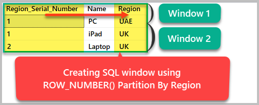
Let's see this in action with our ranking functions.

As you saw in the example, PARTITION BY country told the database to treat artists from the 'United States' as one group, 'Canada' as another, and so on. The ranking was then applied to the artists within each of those country groups. This is an incredibly common and powerful pattern for analysis.

4. Practice: Combining CTEs and Window Functions

A crucial rule to remember is that you cannot use a window function directly in a WHERE or HAVING clause. This is because of the logical order of operations in SQL: the WHERE clause is processed before the window functions are calculated.

So, how do you filter based on a rank, for example, to get the "Top 3"?

This is where your knowledge from the previous lesson comes in handy. The standard professional practice is to:

1. Define a CTE that calculates the rank using a window function.
2. Write the final SELECT statement that queries the CTE and applies a WHERE clause to the newly created rank column.

Let's put this all together in an exercise.

Scenario:
You are an analyst at an e-commerce company. The marketing team wants to know the top two best-selling products (by quantity sold) within each product category.

Tables:

• products (product_id, product_name, category, price)
• orders (order_id, product_id, quantity)

Your Task:
Write a query that returns the category, product_name, and total_quantity_sold for the top 2 products in each category. Use DENSE_RANK() for the ranking.

Steps:

1. First, you need to calculate the total quantity sold for each product. You'll likely need to join orders and products and then GROUP BY product_id, product_name, and category.
2. Create a CTE based on this initial aggregation.
3. Inside the CTE, add a new column using the DENSE_RANK() window function. You want to rank products within each category based on their total quantity sold (in descending order).
4. Finally, write a SELECT statement that queries your CTE and filters for rows WHERE the rank is less than or equal to 2.

WITH ProductSales AS (
    -- Step 1: Calculate total quantity sold for each product
    SELECT
        p.category,
        p.product_name,
        SUM(o.quantity) AS total_quantity_sold
    FROM
        products AS p
    JOIN
        orders AS o ON p.product_id = o.product_id
    GROUP BY
        p.category,
        p.product_name
),
RankedProductSales AS (
    -- Step 2: Rank products within each category based on sales
    SELECT
        category,
        product_name,
        total_quantity_sold,
        DENSE_RANK() OVER (PARTITION BY category ORDER BY total_quantity_sold DESC) AS rnk
    FROM
        ProductSales
)
-- Step 3: Filter for the top 2 ranked products in each category
SELECT
    category,
    product_name,
    total_quantity_sold
FROM
    RankedProductSales
WHERE
    rnk <= 2
ORDER BY
    category,
    total_quantity_sold DESC;

Conclusion

In this lesson, you've added a powerful set of tools to your SQL arsenal. Window functions for ranking are essential for creating leaderboards, finding top performers, de-duplicating data, and much more.

Key Takeaways:

• Window functions perform calculations on a set of rows without collapsing them.
• ROW_NUMBER(), RANK(), and DENSE_RANK() are used for ranking, differing primarily in how they handle ties.
• The PARTITION BY clause is used to create separate "windows" or groups, allowing you to apply functions like RANK() independently to each group.
• You cannot filter on a window function in a WHERE clause. The standard pattern is to calculate the rank in a CTE and then filter on the rank column in the outer query.

In our next lesson, we will continue exploring window functions. We will move beyond ranking to learn how to calculate running totals and moving averages, which are fundamental for trend analysis. This will introduce you to the concept of a "frame clause" (ROWS / RANGE), which gives you even more control over your window.