Mastering CTEs for Cleaner Queries

1. Understanding Common Table Expressions (CTEs)

A CTE is essentially a subquery that you define and name at the beginning of your main query using the WITH keyword. Think of it as creating a temporary, virtual table that exists only for the duration of that single query. This allows you to break down a complex problem into logical, sequential steps, making your code infinitely more readable.

Let's start by understanding the basic definition and syntax.

As the resource explained, the basic syntax is:

WITH CteName (column1, column2) AS (
    -- This is the inner query, just like a subquery
    SELECT
        source_column1,
        source_column2
    FROM your_table
    WHERE condition
)
-- This is the outer query that uses the CTE
SELECT
    column1,
    column2
FROM CteName;

The image below provides a great visual breakdown of this structure.

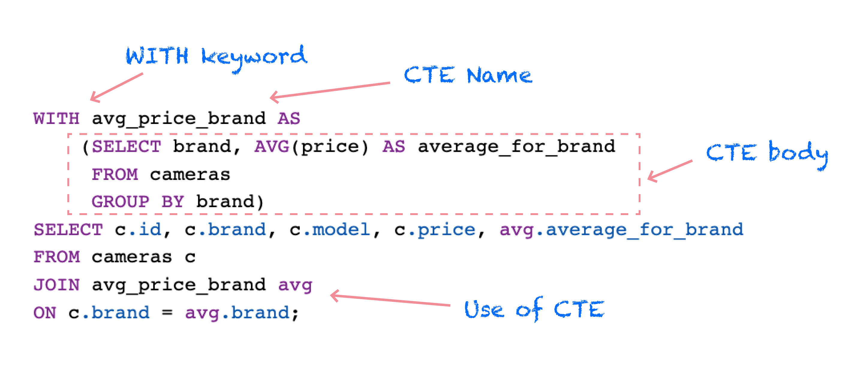
The key takeaway is that you are simply giving a name to a result set, which you can then treat just like any other table in the rest of your query.

2. From Tangled Subqueries to Clean CTEs

Now for the main event: seeing how CTEs transform a complex query. In the previous lesson, you saw how we could nest a subquery in a FROM clause (a derived table) or a WHERE clause. When a problem requires several such steps, the query can become a "query within a query within a query," which is notoriously hard to read.

Let's look at a direct comparison. The following resource shows a query written first with multiple subqueries and then rewritten with CTEs.

The difference is stark. The subquery version is difficult to parse because the logic is inside-out. You have to find the innermost query first and work your way out.

The CTE version, however, exhibits sequential logic:

1. total_by_customer: First, we calculate the total amount for each customer.
2. books_by_customer: Next, we calculate the amount spent on books for each customer.
3. music_by_customer: Then, the amount spent on music.
4. video_by_customer: And the amount spent on videos.
5. Final SELECT: Finally, we join all these named, temporary results together.

This top-down, procedural style makes your logic explicit and far easier for you (and your colleagues) to understand and maintain.

3. Chaining CTEs for Multi-Step Analysis

The real power of CTEs shines when you need to perform a sequence of transformations, where each step builds upon the previous one. You can define multiple CTEs in a single WITH clause, and a later CTE can reference an earlier one.

The syntax for multiple CTEs is:

WITH
Cte1 AS (
    -- First step
    SELECT ... FROM ...
),
Cte2 AS (
    -- Second step, which can use Cte1
    SELECT ... FROM Cte1 ...
),
Cte3 AS (
    -- Third step, which can use Cte1 and/or Cte2
    SELECT ... FROM Cte2 ...
)
-- Final query using one or more of the CTEs
SELECT ... FROM Cte3 ...;

Notice you only use the WITH keyword once. The subsequent CTEs are separated by commas.

Let's see a practical example of this.

This multi-step process is a common pattern in data analysis:

1. Aggregate data to an initial level (e.g., total sales per product).
2. Summarize that aggregation (e.g., average of all product totals).
3. Filter based on the summary (e.g., find products above the average).
4. Present the final result (e.g., rank the filtered products).

Trying to do this with nested subqueries would be extremely confusing. CTEs make the logic clear and organized.

4. Practice Exercise

Let's refactor a problem using CTEs. We'll use the same e-commerce tables from the previous lesson: customers, orders, and products.

Tables:

• customers (customer_id, name, city)
• orders (order_id, customer_id, product_id, quantity, order_date)
• products (product_id, product_name, price)

Your Task:
Write a SQL query to find the name and total spending of customers who have purchased a product from the 'Electronics' category.

A solution using subqueries might look like this (don't run this, just read it):

-- Messy subquery version
SELECT
    c.name,
    SUM(p.price * o.quantity) AS total_spending
FROM
    customers c
JOIN
    orders o ON c.customer_id = o.customer_id
JOIN
    products p ON o.product_id = p.product_id
WHERE
    c.customer_id IN (
        SELECT DISTINCT o.customer_id
        FROM orders o
        JOIN products p ON o.product_id = p.product_id
        WHERE p.category = 'Electronics'
    )
GROUP BY
    c.customer_id, c.name;

This is not terrible, but the logic is split between a subquery and the main query.

Now, rewrite this query using CTEs to make the logic more sequential and clear.

Hints:

1. Create a first CTE named electronic_customers that finds the customer_id of everyone who bought an 'Electronics' product.
2. In your main query, join the customers, orders, and products tables, but also join to your electronic_customers CTE on customer_id to filter for only those customers.
3. Calculate the total spending and group by the customer.

WITH electronic_customers AS (
    -- Step 1: Identify all customers who have purchased an electronics item
    SELECT DISTINCT
        o.customer_id
    FROM
        orders AS o
    JOIN
        products AS p ON o.product_id = p.product_id
    WHERE
        p.category = 'Electronics'
)
-- Step 2: Calculate total spending for ONLY those customers
SELECT
    c.name,
    SUM(p.price * o.quantity) AS total_spending
FROM
    customers AS c
JOIN
    orders AS o ON c.customer_id = o.customer_id
JOIN
    products AS p ON o.product_id = p.product_id
JOIN
    electronic_customers AS ec ON c.customer_id = ec.customer_id
GROUP BY
    c.customer_id, c.name
ORDER BY
    total_spending DESC;

Conclusion

Excellent work. You have now learned one of the most important techniques for writing professional, scalable, and maintainable SQL. By moving beyond nested subqueries to CTEs, you are adopting a style of coding that emphasizes clarity and logical structure.

Key Takeaways:

• CTEs are temporary, named result sets defined using the WITH keyword.
• Their primary benefit is improving the readability and structure of complex queries by breaking them into logical, sequential steps.
• You can chain multiple CTEs together, allowing a later CTE to reference an earlier one, which is perfect for multi-stage data transformations.
• While CTEs and subqueries can often achieve the same result, CTEs are generally preferred for any query with more than one logical step.

In our next lesson, we will explore window functions. These functions, such as ROW_NUMBER(), RANK(), and SUM() OVER (...), perform calculations across a set of table rows. They are a perfect partner to CTEs, as you can first use a CTE to prepare and structure your data, and then apply window functions in the final SELECT statement to perform sophisticated rankings, running totals, and comparisons.