Window Functions: Running Totals & Moving Averages with Frame Clauses

1. Running Totals: Accumulating Values Over Time

A running total, or cumulative sum, calculates the sum of a value up to the current row in the ordered set. It’s perfect for tracking progress over time, like year-to-date (YTD) sales.

In the last lesson, we used PARTITION BY to create our windows. When calculating a running total, the ORDER BY clause inside OVER() is the most critical part. It tells SQL the sequence in which to accumulate the values.

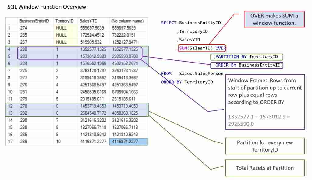
The basic syntax for a running total is surprisingly simple:

SUM(value_column) OVER (ORDER BY date_column)

You might wonder: how does SQL know to sum everything up to the current row and not the entire column? It does this by using a default window frame. When you use ORDER BY with an aggregate window function, SQL implicitly adds the following frame clause:

ROWS BETWEEN UNBOUNDED PRECEDING AND CURRENT ROW

This means: "for each row, sum the values from the very first row in the partition up to and including the current row."

Let's see this in action.

As you saw, combining SUM(...) OVER(...) with PARTITION BY is powerful. You can calculate YTD sales for each product category, cumulative user activity for each country, and more—all in a single, clean query.

2. Moving Averages: Smoothing Trends with Explicit Frames

While running totals accumulate values indefinitely, a moving average (or rolling average) calculates the average of a value over a specific, sliding window of a fixed size (e.g., the last 7 days). This is extremely useful in data analysis and BI because it smooths out short-term volatility, making it easier to spot underlying trends.

To calculate a moving average, we must explicitly define the window frame. We can no longer rely on the default. For an N-period moving average, the syntax is:

ROWS BETWEEN (N-1) PRECEDING AND CURRENT ROW

For example, a 7-day moving average would use ROWS BETWEEN 6 PRECEDING AND CURRENT ROW (6 previous rows + the current row = 7 total rows).

Let's turn to a resource that has excellent visuals for understanding how these frames work.

Now that you have a solid visual understanding of frames, let's see the full SQL syntax for moving averages.

3. ROWS vs. RANGE: A Crucial Distinction

So far, we have only used ROWS in our frame clause. ROWS defines a frame based on a specific number of physical rows relative to the current one. However, there's another option: RANGE.

RANGE defines a frame based on a logical range of values in the ORDER BY column relative to the current row's value. This is particularly useful when dealing with date or time-series data that might have gaps.

• ROWS BETWEEN 6 PRECEDING AND CURRENT ROW: "Look at the 6 rows that come before this one, regardless of their date." If you have data missing for 3 days, it will still just grab the 6 previous available data points.
• RANGE BETWEEN INTERVAL '6 days' PRECEDING AND CURRENT ROW: "Look at all rows whose date is within the last 6 days from the current row's date." If you have missing days, this window will contain fewer than 7 rows.

Let's see the syntax for RANGE.

The exact syntax for date/time intervals can vary slightly between SQL dialects (e.g., DATE_SUB in MySQL or DATEADD in SQL Server), but the RANGE concept remains the same.

4. Practice Exercise

It's time to put these concepts into practice. Imagine you are analyzing sales data for a retail company. You have a table named daily_sales with the following structure:

• sale_date (DATE)
• store_id (INTEGER)
• daily_revenue (DECIMAL)

Your Task:
Write a single SQL query that returns the sale_date, store_id, and daily_revenue, along with two new columns:

1. cume_revenue_by_store: The cumulative (running total) of revenue for each store, ordered by date.
2. moving_avg_7day: The 7-day moving average of revenue for each store.

Instructions:

• You will need to partition your calculations by store_id.
• Both calculations should be ordered by sale_date.
• For the moving average, define a frame that includes the current day and the 6 preceding days.

Take a moment to construct your query. Think about which functions to use and how to define the OVER() clause for each calculation.

SELECT
    sale_date,
    store_id,
    daily_revenue,

    -- 1. Cumulative revenue for each store
    SUM(daily_revenue) OVER (
        PARTITION BY store_id
        ORDER BY sale_date
        -- Implicit frame: ROWS BETWEEN UNBOUNDED PRECEDING AND CURRENT ROW
    ) AS cume_revenue_by_store,

    -- 2. 7-day moving average of revenue for each store
    AVG(daily_revenue) OVER (
        PARTITION BY store_id
        ORDER BY sale_date
        ROWS BETWEEN 6 PRECEDING AND CURRENT ROW
    ) AS moving_avg_7day

FROM
    daily_sales
ORDER BY
    store_id,
    sale_date;

Conclusion

In this lesson, you've significantly expanded your capabilities with window functions, moving from ranking to powerful time-series aggregations. These are not just theoretical exercises; running totals and moving averages are workhorse calculations used daily in finance, marketing, and operations analysis.

Key Takeaways:

• Running Totals are typically calculated with SUM(...) OVER (ORDER BY ...) and use a default frame of ROWS BETWEEN UNBOUNDED PRECEDING AND CURRENT ROW.
• Moving Averages are calculated with AVG(...) OVER (ORDER BY ...) and require an explicit frame, such as ROWS BETWEEN (N-1) PRECEDING AND CURRENT ROW.
• The Frame Clause gives you precise control over which rows are included in a window function's calculation.
• ROWS defines a frame by physical row count, while RANGE defines it by a value offset, which is useful for handling gaps in time-series data.
• Both calculations can be combined with PARTITION BY to apply them independently to different groups of data.

In our next and final lesson for this module, we will explore a different aspect of SQL: how to combine the results of two or more SELECT statements using the set operators UNION, INTERSECT, and EXCEPT.