Sampling Schemes: A Comparative Analysis

From Distributions to Sampling Schemes

In the previous lesson, you reviewed the Binomial distribution, which models k successes in n trials when there are two possible outcomes. The Multinomial distribution is a direct extension of this concept. It applies when each trial has more than two possible outcomes.

Imagine sorting n subjects into J different categories. The Multinomial distribution gives you the probability of observing a specific count (n_1, n_2, ..., n_J) in each category.

Now, let's see how these distributions form the basis for the three main sampling schemes for contingency tables.

The Core Idea: What Was Fixed in the Study Design?

When you encounter a problem with a contingency table, the most important question you can ask to identify the sampling scheme is:

"Which totals in the table were fixed by the researcher before collecting the data?"

The answer to this question is your primary decision rule. Let's explore the three possibilities.

1. Poisson Sampling: No Totals are Fixed

In a Poisson sampling scheme, the researcher doesn't fix any totals in advance—not the row totals, not the column totals, and not even the grand total. Instead, they observe events over a fixed window of time or space and simply count how many fall into each cell of the contingency table.

• How to spot it: The study description will imply an observation period, and there will be no mention of a pre-determined sample size. The total number of subjects, n, is a random outcome itself.
• The underlying model: The count in each cell ($n_{ij}$) is treated as an independent random variable from a Poisson distribution.
• Example: A hospital administrator observes the emergency room for 24 hours and classifies each arriving patient by severity (High, Low) and insurance status (Insured, Uninsured). The total number of patients who show up is not known beforehand.

The resource you just read describes this scenario. Read the short section on Poisson sampling and its accompanying example to solidify this idea.

Decision Rule: If the study involves counting events over time/space and the total count is random, it's Poisson sampling.

2. (Single) Multinomial Sampling: Only the Grand Total is Fixed

This is a very common design. A researcher decides on a total sample size, n, takes a single random sample from a population, and then classifies each individual based on two categorical variables simultaneously.

• How to spot it: The study description will explicitly state that a single sample of size n was taken. The row and column totals are random outcomes; only the grand total n was fixed.
• The underlying model: The IJ cell counts in the table are considered a single outcome from one large Multinomial distribution with n trials.
• Example: A researcher surveys n=1000 randomly selected voters and asks each person for their political affiliation (Variable 1) and their opinion on a policy (Variable 2). The grand total is fixed at 1000, but the number of people in each political party or holding each opinion is unknown until the data is collected.

The following image and its description provide a perfect example of this.

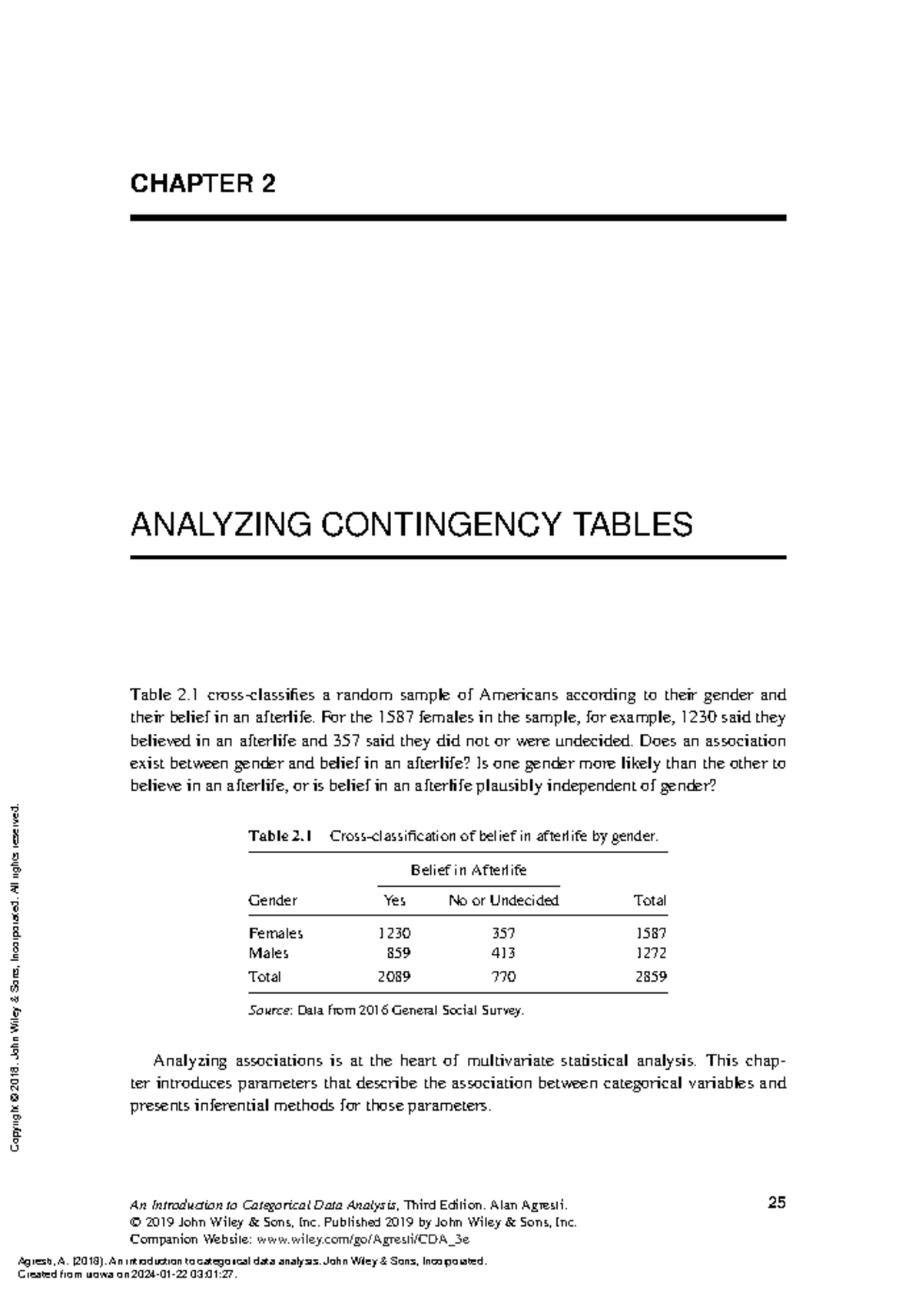
Based on the description "a random sample of Americans" was taken and then "cross-classified", we can conclude this is (Single) Multinomial sampling.

Now, let's look at how the resources define this scheme.

Decision Rule: If the study takes one random sample of a fixed size n and classifies individuals on two variables, it's (Single) Multinomial sampling.

3. Product Multinomial Sampling: Row or Column Totals are Fixed

In this design, the researcher identifies distinct populations (the categories of one variable) and then takes a separate random sample from each one. Here, the totals for one dimension of the table (either the rows or the columns) are fixed before data collection. This is also called Independent Multinomial sampling.

• How to spot it: The study description will say that separate samples were taken from different groups. For example, "we sampled 100 smokers and 200 non-smokers" or "we sampled 200 people from City A, 150 from City B, and 300 from City C."
• The underlying model: We have independent multinomial samples for each row (or column). If the response variable for each group has only two categories, it simplifies to independent binomial samples.
• Example: A researcher wants to compare the effectiveness of two drugs. They recruit 100 patients for Drug A and 100 patients for Drug B. The row totals (100, 100) are fixed. They then observe the outcome for each group (Improved, Did not improve). The column totals are random.

Let's see how our resources describe this scheme, often in the context of testing for "homogeneity."

Decision Rule: If the study takes separate random samples from groups defined by one variable, it's Product Multinomial sampling.

Putting It All Together: A Worked Example

It's crucial to understand that the same table of numbers could have been generated by different sampling schemes. Identifying the correct one depends entirely on the study's description.

The following example walks through this exact scenario. It is excellent practice for the exam.

This distinction is not just academic. As one of our resources notes, "the tests for homogeneity of proportions and independence are exactly the same. However, the sampling methods and hypotheses are different." Getting this first step right is essential.

Conclusion

In this lesson, you learned how to distinguish between the three main sampling schemes for contingency tables by asking one key question: What totals were fixed by the study design?

Here are your key takeaways and decision rules:

• Poisson Sampling: No totals are fixed. The grand total n is random. You are counting events in a fixed window.
• (Single) Multinomial Sampling: Only the grand total n is fixed. You take one sample and classify it on two variables.
• Product (Independent) Multinomial Sampling: Row or column totals are fixed. You take separate samples from predefined groups.

Mastering this distinction is the first step toward choosing the correct analysis.

In the next lesson, we will build on this foundation. You'll learn how the sampling scheme you've identified determines whether you should calculate and compare row percentages or column percentages in your contingency table, which is a common task in applied problems. This will also lead us to formulating the correct null hypothesis for our statistical test.