Introduction
Hello! Welcome to your intensive course on categorical data analysis and generalized linear models. Given your tight timeline for the midterm, we'll move quickly, focusing on the concepts and applications you'll need to recognize and solve exam problems.
Today, we'll start with a foundational review. As you requested, this first lesson will refresh your memory on three essential probability distributions: the Binomial, Poisson, and Normal distributions. Your goal is to be comfortable with their key properties—specifically their probability mass/density functions (PMF/PDF), mean, and variance.
A solid grasp of these distributions is critical. They are not just abstract concepts; they are the building blocks for almost everything that follows in this course, from the sampling schemes we'll discuss next to the structure of the Generalized Linear Models (GLMs) that are a major part of your exam.
Binomial Distribution
The Binomial distribution is used to model the number of "successes" in a fixed number of independent trials. Think of it as the result of a series of repeated, identical experiments where each experiment has only two possible outcomes (e.g., heads/tails, success/failure, yes/no).
To understand the conditions under which a scenario can be modeled with a Binomial distribution, watch the first part of the following video. It introduces a helpful acronym, "BINS," which is useful for quickly identifying these situations on an exam.
Binomial Distribution EXPLAINED with Examples
This video from Ace Tutors explains the four conditions that define a binomial experiment.
Watch the section from the beginning until 2:11, which covers the 'BINS' criteria: Binary outcomes, Independent trials, N number of trials, and Same probability of success.
As the video explained, a random variable follows a Binomial distribution if:
- Binary: Each trial has only two outcomes (success/failure).
- Independent: The outcome of one trial does not affect others.
- Number of trials is fixed ().
- Same probability of success () for each trial.
The variable then represents the total count of successes in those trials.
Now, let's look at the formulas for its key properties. The next part of the video breaks down the probability formula and then discusses the mean and variance.
Binomial Distribution EXPLAINED with Examples
Continue with the same video to see how to calculate probabilities, the mean, and the variance.
Watch from 2:11 to 8:34. This segment explains the probability mass function (PMF), the mean, and the standard deviation with a clear, worked example.
To summarize, here are the key properties for a Binomial random variable :
-
Probability Mass Function (PMF): The probability of observing exactly successes in trials.
where is the number of ways to choose successes from trials.
-
Mean (Expected Value): The average number of successes you'd expect.
-
Variance: A measure of the spread of the distribution.
Keep these formulas handy. You'll need them to understand binomial sampling in our next lesson.
Poisson Distribution
Next, we'll review the Poisson distribution. While the Binomial distribution counts successes in a fixed number of trials, the Poisson distribution models the number of events occurring within a fixed interval of time or space. The key is that we know the average rate () at which events occur, but there isn't a fixed number of "trials." For instance, it could model the number of emails you receive in an hour or the number of defects in a square meter of fabric.
This video provides a great introduction to the concept and its properties.
Data Science & Statistics Tutorial: The Poisson Distribution
This video from 365 Data Science clearly explains the Poisson distribution, its parameter lambda, its PMF, and its mean and variance.
Watch from the beginning to 4:42. Focus on what lambda represents, the PMF formula, and the unique relationship between the mean and variance.
As the video highlighted, the key properties for a Poisson random variable are straightforward:
-
Probability Mass Function (PMF): The probability of observing exactly events in an interval.
Here, is the average number of events in that interval, and is Euler's number ().
-
Mean (Expected Value): The average number of events is simply .
-
Variance: The variance is also .
The fact that the mean equals the variance is a defining feature of the Poisson distribution. This is a critical diagnostic property you can use on an exam. If you're given descriptive statistics for a dataset and see that the sample mean is very close to the sample variance, it's a strong hint that a Poisson distribution might be a good model for the data.
Normal Distribution
Finally, let's review the Normal (or Gaussian) distribution. Unlike the Binomial and Poisson distributions which are for discrete count data, the Normal distribution is for continuous data (e.g., height, weight, temperature). Its famous symmetric, bell-shaped curve is defined by its mean () and variance ().
For a quick and effective review, we'll use a reference sheet. It gets straight to the point, which is ideal for exam preparation.
This 'Probability Cheatsheet' provides a very concise summary of many distributions. We'll use it to quickly review the Normal distribution.
First, read the section on the 'Normal Distribution' (page 2) to remind yourself of its key characteristics. Then, find the 'Table of Distributions' at the end of the document and locate the row for the Normal distribution to see its PDF, mean, and variance formulas in one place.
The cheatsheet gives you everything you need. Here are the key properties for a Normal random variable :
-
Probability Density Function (PDF): Describes the shape of the bell curve.
You likely won't need to manually integrate this on an exam, but you should recognize its form and know that centers the curve and controls its spread.
-
Mean (Expected Value): The center of the distribution.
-
Variance: The measure of the spread or width of the bell curve.
Summary and Key Differences
To help you quickly decide which distribution might be appropriate for a given problem, here is a summary table. This kind of mental checklist is invaluable for an exam.
| Feature | Binomial Distribution | Poisson Distribution | Normal Distribution |
|---|---|---|---|
| Data Type | Discrete (counts) | Discrete (counts) | Continuous |
| Description | Number of successes in fixed trials. | Number of events in a fixed interval. | Measurements of a continuous quantity. |
| Parameters | (number of trials), (probability of success) | (average rate of events) | (mean), (variance) |
| Mean | |||
| Variance | |||
| Key Hint | Fixed number of trials, two outcomes. Var < Mean. | An average rate over time/space. Var = Mean. | Bell-shaped, symmetric. For continuous measurements. |
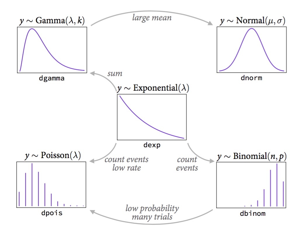
The following image provides a great visual map of how these distributions (and others) relate to each other. For now, just focus on the Binomial, Poisson, and Normal shapes and parameters. Notice the arrow from Binomial to Poisson, which represents that the Poisson distribution can approximate the Binomial when is large and is small.
Conclusion
In this lesson, we completed a rapid review of the Binomial, Poisson, and Normal distributions. You should now be comfortable with:
- The "story" behind each distribution—what kind of data it models.
- The key parameters that define each distribution (; ; ).
- The formulas for the mean and variance of each.
- The crucial diagnostic hint for the Poisson distribution: its mean is equal to its variance.
This foundation is essential for our next lesson, where we will examine sampling schemes. You'll learn how study designs lead to data that can be modeled by these very distributions, which in turn determines the correct way to set up a contingency table and formulate a hypothesis.