Introduction
Welcome back! In the previous lesson, we established a crucial skill: identifying the sampling scheme of a study (Poisson, Multinomial, or Product Multinomial) by determining which totals in a contingency table were fixed by the research design.
Today, we will apply that skill to achieve two practical goals essential for your exam:
- Constructing a contingency table to organize categorical data.
- Making the critical decision of whether to use row or column percentages for comparison.
This lesson is all about moving from raw counts to meaningful comparisons. The choice of percentages is not arbitrary; it's dictated by the study design you learned to identify. Getting this right is the foundation for correctly interpreting relationships and, as we'll see next, for choosing the right hypothesis test.
What is a Contingency Table?
A contingency table (or cross-tabulation) is simply a grid that displays the frequency distribution of two or more categorical variables. It allows us to see how the categories of one variable are "contingent on" the categories of another.
Let's look at the basic structure and a real-world example.
[PDF] STAT 705: Analysis of Contingency Tables
This resource from the University of South Carolina provides a clear, formal definition of a contingency table and its notation.
Please read the sections 'Contingency tables & their distributions' (page 2) and 'Abstract contingency table' (page 3). Then, review the 'Example of 3x3 table' on page 4, which shows how data from a study on knee injuries is organized.
As you saw, the table organizes individuals into cells based on their classification for two variables (e.g., Injury Type and Surgical Result). Each cell, , contains the count of individuals in row i and column j. We also have row totals (), column totals (), and a grand total ().
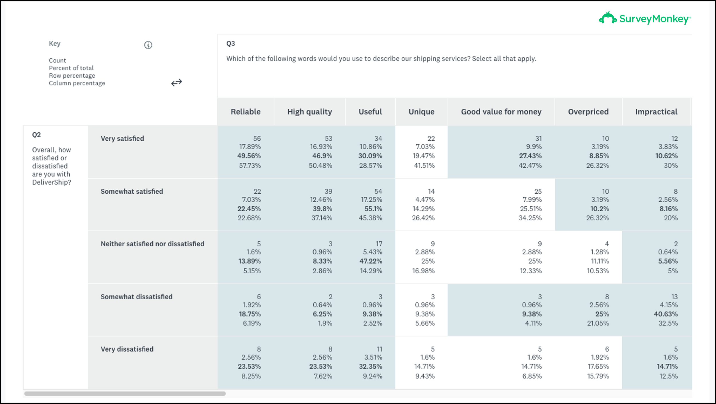
Why We Need Percentages
Raw counts can be misleading, especially when comparing groups of different sizes. For example, if Group A has 80 successes and Group B has 40, it's tempting to say Group A is better. But if Group A had 100 people and Group B had only 40, their success rates would be 80% and 100%, respectively. Percentages standardize our comparisons.
The main question is: should you calculate percentages based on row totals or column totals?

The Decision Rule: Explanatory vs. Response Variables
Here is the core principle that will guide you on the exam:
Calculate percentages within the categories of the explanatory (independent) variable so that you can compare the distribution of the response (dependent) variable across those categories.
The sampling scheme you identified in the last lesson is what tells you which variable is explanatory.
Case 1: Product Multinomial Sampling (Fixed Row or Column Totals)
This is the most straightforward case.
- Recap: In this design, the researcher fixes the sample sizes for the categories of one variable before collecting data. For example, they decide to survey 100 smokers and 100 non-smokers.
- Decision: The variable with the fixed totals is the explanatory variable.
- If row totals were fixed, calculate row percentages.
- If column totals were fixed, calculate column percentages.
Let's see this in action with two classic examples: a clinical trial and a case-control study.
[PDF] STAT 705: Analysis of Contingency Tables
This reading provides perfect examples of product multinomial sampling. Pay close attention to what was fixed in each study design and how that dictates the comparison.
Read the sections 'Product multinomial table' (page 6), 'Clinical trial example' (page 7), and 'Case-control studies' (page 9). For each example, ask yourself: What totals were fixed by the design? Which variable is therefore explanatory? Does this mean I should compare numbers across rows or down columns?
Let's break down what you just read:
-
Clinical Trial Example (Aspirin vs. Placebo):
- What was fixed? The number of physicians in the Placebo group () and the Aspirin group (). The row totals were fixed.
- Explanatory Variable: The row variable (Group: Placebo/Aspirin).
- Decision: We must use row percentages. We would calculate
18/11034,171/11034, etc., to compare the percentage of fatal attacks, nonfatal attacks, and no attacks between the aspirin and placebo groups.
-
Case-Control Study Example (Smoking and Lung Cancer):
- What was fixed? The number of Cases () and Controls (). The column totals were fixed.
- Explanatory Variable: The column variable (Group: Case/Control).
- Decision: We must use column percentages. We would calculate
688/709and21/709to compare the proportion of smokers and non-smokers within the cancer group, and then compare that to the proportions in the control group.
Case 2: (Single) Multinomial or Poisson Sampling (Only Grand Total Fixed or No Totals Fixed)
This case is more flexible because the study design doesn't force one variable to be explanatory.
- Recap: A single sample is taken and cross-classified on two variables (Multinomial), or events are counted over a period (Poisson).
- Decision: Your choice depends on the research question. You must decide which variable you want to treat as a predictor (explanatory) and which you want to treat as an outcome (response).
[PDF] Chapter 5 - Log-Linear Models for Contingency Tables
This resource directly addresses the choice you have when the sampling scheme doesn't pre-determine the explanatory variable. It frames this as choosing between a symmetric or asymmetric analysis.
Read the paragraph on page 9 that begins 'Note that if the total is fixed and the sampling scheme is multinomial...'. Focus on the distinction between treating variables 'symmetrically' (studying correlation) versus 'asymmetrically' (predictor and response).
As the reading suggests, when you have a single multinomial sample, you can choose your approach.
- Example: Consider the Framingham Heart Study data from the resource (LINK, Table 5.1). We have a single sample of 1329 patients classified by Cholesterol level and Heart Disease status.
- Research Question: "Does high cholesterol increase the risk of heart disease?"
- Explanatory Variable: Cholesterol Level (the presumed cause/predictor). This is the row variable.
- Response Variable: Heart Disease (the outcome). This is the column variable.
- Decision: Since the explanatory variable is in the rows, we calculate row percentages. We would compare the percentage of people with heart disease in the
< 260cholesterol group (51/1043 = 4.9%) to the percentage in the260+group (41/286 = 14.3%). This allows for a direct comparison of risk.
Worked Application
Let's apply this logic to a typical exam-style problem.
Problem: A researcher wants to know if there is an association between the operating system a developer uses (macOS, Windows, Linux) and their primary programming language (Python, JavaScript, Java). They survey a random sample of 500 developers from a large tech conference and obtain the following counts:
| OS | Python | JavaScript | Java | Total |
|---|---|---|---|---|
| macOS | 60 | 80 | 30 | 170 |
| Windows | 50 | 90 | 70 | 210 |
| Linux | 60 | 20 | 40 | 120 |
| Total | 170 | 190 | 140 | 500 |
Question: What percentages should you calculate to determine if the choice of programming language depends on the operating system?
Solution Steps:
-
Identify the sampling scheme: A "random sample of 500 developers" was taken and then classified on two variables (OS and Language). Only the grand total was fixed. This is (Single) Multinomial Sampling.
-
Identify explanatory/response variables: The question asks if "language depends on the operating system." This implies:
- Explanatory Variable: Operating System (OS)
- Response Variable: Programming Language
-
Apply the decision rule: We must calculate percentages within the categories of the explanatory variable (OS). Since OS is the row variable, we calculate row percentages.
-
Perform the calculation:
- macOS:
- Python:
60/170 = 35.3% - JavaScript:
80/170 = 47.1% - Java:
30/170 = 17.6% - Total: 100%
- Python:
- Windows:
- Python:
50/210 = 23.8% - JavaScript:
90/210 = 42.9% - Java:
70/210 = 33.3% - Total: 100%
- Python:
- Linux:
- Python:
60/120 = 50.0% - JavaScript:
20/120 = 16.7% - Java:
40/120 = 33.3% - Total: 100%
- Python:
- macOS:
Conclusion: By calculating row percentages, we can now easily compare the language preferences across OS users. For instance, we can see that Python is most popular among Linux users (50.0%), while JavaScript is most popular among macOS users (47.1%).
Conclusion
In this lesson, you've learned how to construct and, more importantly, how to correctly interpret a contingency table. You now have a clear, application-focused decision rule for your exam.
Key Takeaways:
- Decision Rule: Always calculate percentages within the levels of the explanatory variable.
- Product Multinomial Sampling: The variable with the fixed totals is your explanatory variable. If row totals are fixed, use row percentages. If column totals are fixed, use column percentages.
- Single Multinomial / Poisson Sampling: Your research question determines the explanatory variable. Decide which variable is the predictor and which is the outcome, then calculate percentages accordingly.
In our next lesson, we will take the final step before running a test. We will use our knowledge of sampling schemes to formulate the correct null hypothesis—either a test of independence or a test of homogeneity. This will tie together everything we've learned in this module.