Binary Logistic Regression: Model and Assumptions

1. Why Can't We Just Use Linear Regression?

Let's start with a motivating question. Imagine we want to model whether a student passes an exam (a binary outcome: Pass=1, Fail=0) based on the number of hours they studied (a continuous predictor). Your first instinct might be to use a simple linear regression model, which you're likely familiar with from your background. However, this approach has some fundamental problems when the outcome is binary.

The video below explains these limitations clearly. It's important to understand why we need a new type of model.

To summarize the key issues of using linear regression for a binary outcome:

1. Unbounded Predictions: A linear regression line can extend infinitely, producing predicted values greater than 1 or less than 0. These are meaningless as probabilities, which must be between 0 and 1.
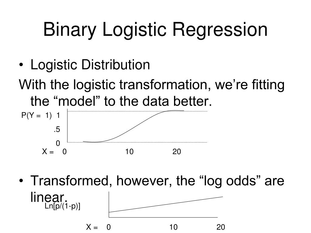
2. Non-Linear Relationship: The relationship between a predictor and the probability of a binary outcome is rarely a straight line. It often follows an "S"-shaped curve (a sigmoid curve). The probability changes slowly at very low and very high values of the predictor and changes most rapidly in the middle.
3. Violation of Homoscedasticity: Linear regression assumes that the variance of the error term is constant. For a binary variable, the variance is $p(1-p)$, where $p$ is the probability of the event. Since $p$ changes with the predictors, the variance is not constant, which violates a key assumption and makes standard errors unreliable.

These problems show that linear regression is the wrong tool for the job. We need a model that is designed to handle probabilities—a Generalized Linear Model.

2. The Logistic Regression Model

Logistic regression solves these problems by using a specific link function to connect the linear predictor to the outcome probability.

Let's build the model step-by-step. The video below does an excellent job of starting with the problems of linear regression and logically building up to the final logistic regression equation.

Let's formalize the key equations from the video.

Step 1: Modeling Probability with the Logistic Function

We model the probability of the outcome being 1, $P(Y=1)$, written as $p$, using the logistic function:

This S-shaped function guarantees that the predicted probability $p$ will always be between 0 and 1, solving the main issue with linear regression. However, the relationship between $X$ and $p$ is non-linear, making it hard to interpret the coefficient ${\beta }_1$.

Step 2: The Logit Transformation (Probability -> Odds -> Log-Odds)

To get a linear model, we transform the left side of the equation.

First, we move from probability to odds. The odds of an event are the ratio of the probability that the event occurs to the probability that it does not occur.

If you substitute the logistic function formula for $p$ into this odds equation, the math simplifies beautifully to:

We're almost there! This is still an exponential, not a linear, relationship. To linearize it, we take the natural logarithm (ln) of both sides. This gives us the log-odds, which is also called the logit.

This is the equation for a binary logistic regression model.

The expression $\ln (p/(1-p))$ is the logit link function. It "links" the probability of the outcome to the linear predictor on the right-hand side. This transformation is the core of logistic regression and allows us to use a linear model framework for a binary outcome.

The image below provides a great visual summary of this transformation.

3. Key Assumptions of Logistic Regression

Just like any statistical model, logistic regression relies on a set of assumptions for its results to be valid and reliable. For an exam, you should be able to list and briefly explain them.

Here is a visual summary of the key assumptions, which can be a helpful memory aid for your exam.

Let's detail the most critical ones:

1. Binary Outcome: The dependent variable must be categorical with only two possible outcomes (e.g., Yes/No, 1/0, True/False).
2. Independence of Observations: The individual observations in your dataset must be independent of each other. This is a design-based assumption; for example, data from the same patient over time would violate this.
3. No Perfect Multicollinearity: The independent variables should not be perfectly correlated with each other. High correlation can destabilize the model and make coefficient estimates unreliable.
4. Linearity in the Logit: This is a crucial assumption. It states that there must be a linear relationship between any continuous independent variables and the log-odds of the outcome. You can check this with scatterplots of the predictor against the logit of the outcome.
5. Large Sample Size: Logistic regression uses Maximum Likelihood Estimation (MLE), which is a "large sample" technique. The reliability of the model, particularly for hypothesis tests (like the Wald and LRT tests you just studied), depends on having a sufficiently large sample.

Conclusion

In this lesson, you've established the foundation for understanding logistic regression. You now know not only why it's necessary but also the mechanics of how it works and the rules it must follow.

Key Takeaways:

• Linear regression is not appropriate for binary outcomes due to unbounded predictions and violated assumptions.
• Logistic regression models the probability of an outcome using a sigmoid (logistic) function, ensuring predictions stay between 0 and 1.
• The model equation is written in terms of log-odds (the logit) to achieve a linear relationship with the predictors: $\ln \left(\frac{p}{1-p}\right)={\beta }_0+{\beta }_{1}X+\dots$.
• The logit link function is what connects the probability to the linear predictor.
• Key assumptions include a binary outcome, independence of observations, no perfect multicollinearity, and a linear relationship between continuous predictors and the log-odds of the outcome.

In our next lesson, we will build directly on this foundation to answer a critical practical question: How do we interpret the intercept (${\beta }_0$) and the regression coefficients (${\beta }_1$, etc.)? This will involve working with odds and odds ratios, which are essential for communicating the results of a logistic regression analysis.