Likelihood Ratio, Wald, and Score Tests: A Comparative Analysis

Hello! Welcome to the final lesson in our module on hypothesis testing in Generalized Linear Models (GLMs).

Over the last three lessons, we've individually covered the "big three" hypothesis tests used in GLMs: the Likelihood Ratio Test (LRT), the Wald test, and the Score test. You've learned the basic purpose and procedure for each one.

Now, we'll bring it all together. Your goal for this lesson is to compare the properties of the Likelihood Ratio, Wald, and Score tests and identify when each is most appropriate. This is a critical skill for your exam, as you'll often need to choose the right tool or interpret results from any of these tests.

1. Three Tests, One Goal, Three Approaches

All three tests—LRT, Wald, and Score—are designed to test hypotheses about model parameters, typically by comparing a simpler (restricted) model to a more complex (full) model. While their goal is the same, they approach it from different perspectives, which affects both their computation and their reliability.

Let's start by consolidating your understanding of how each test works.

How are the likelihood ratio, Wald, and Lagrange multiplier (score ...

The UCLA Statistics page you've seen before has an excellent section that summarizes and compares the three tests. It also includes a helpful diagram.

Please read the introduction (first paragraph), the short section 'The likelihood', and the final section, 'A comparison of the three tests'. Pay close attention to the diagram in the final section, which visually summarizes the differences.

To reinforce this, here is another clear diagram illustrating the core idea:

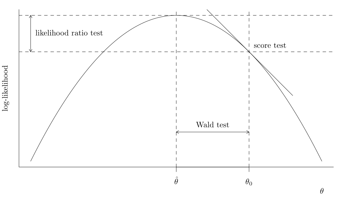
Visual Comparison of Likelihood Ratio, Wald, and Score Tests — This diagram shows the log-likelihood function for a single parameter $\theta$. The **LRT** measures the vertical difference in height between the function at the MLE ($\hat{\theta}$) and at the null value ($\theta_0$). The **Wald test** measures the horizontal distance between $\hat{\theta}$ and $\theta_0$. The **Score test** measures the slope (gradient) of the function at $\theta_0$.

Let's summarize the key computational difference, which is a common exam topic:

Test	What it Requires	Analogy
Likelihood Ratio (LRT)	Fit both the full and restricted models.	To see how much better the view is from the top of the mountain vs. a lower ledge, you have to visit both spots.
Wald Test	Fit only the full model.	You're at the top of the mountain and estimate how far you are from a specific point (the null hypothesis) on the ground.
Score Test	Fit only the restricted model.	You're on a ledge (the null hypothesis) and look at the slope. If it's steep, you know the peak is far away.

2. Asymptotic Equivalence vs. Finite Sample Performance

A key theoretical property is that the LRT, Wald, and Score tests are asymptotically equivalent. This means that as the sample size grows infinitely large, their test statistics and p-values will converge to the same values.

This image shows a simulation of this convergence. Notice how the three lines (red for LRT, green for Score, blue for Wald) become nearly identical in the plots with larger sample sizes (e.g., n0 = 10000).

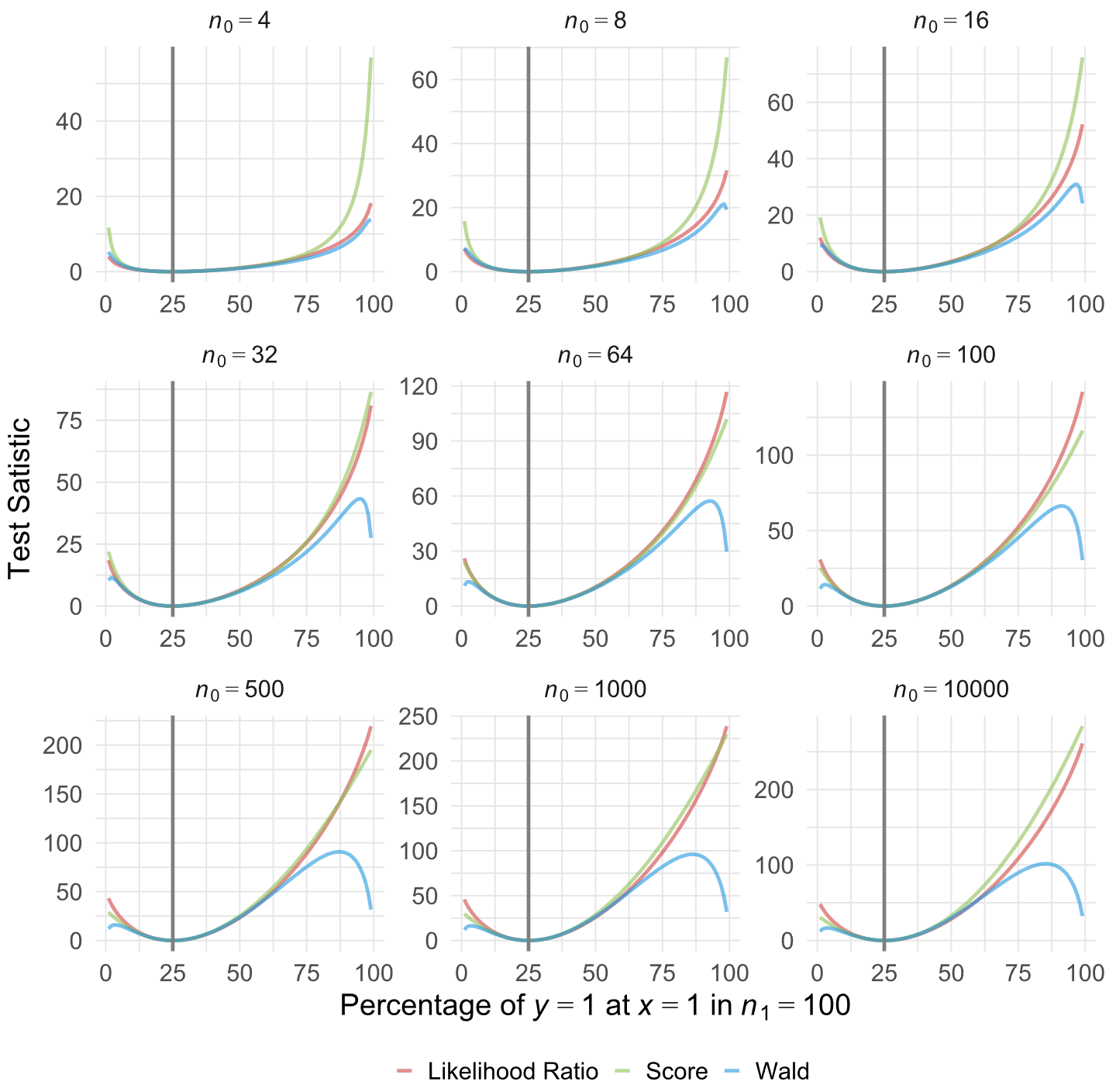
Comparison of Likelihood Ratio, Score, and Wald Test Statistics Across Sample Sizes — This grid of plots shows the test statistics for the LRT, Score, and Wald tests across different sample sizes (n0). As n0 increases, the three test statistics become much more similar, illustrating their asymptotic equivalence.

However, for your exam, you'll be dealing with finite samples, where the results can and do differ. This is where knowing their properties becomes crucial.

3. Which Test to Trust? Reliability and Common Pitfalls

When results from the three tests differ, which one should you rely on? The general consensus is that the LRT is the most reliable, while the Wald test can be the least reliable, especially in certain situations.

The following reading from Stack Exchange provides excellent insight into why this is the case.

Likelihood ratio vs. score vs. Wald test: Different p values, which to ...

This discussion thread provides a clear, practical explanation of why the tests can give different p-values and which one to trust, quoting a leading expert in categorical data analysis.

Please read the following three sections of the top answer: Start with the first paragraph of the first answer (by user jsakaluk), focusing on the quote from Agresti regarding the Wald test's reliability in small samples. Then read the next answer (by user DrJerryTAO) which discusses the 'Hauck-Donner effect' and why the Wald test can fail with very large effects or data separation. Finally, read the section on the Likelihood-ratio test, which explains why it is generally more robust.

Let's break down the key takeaways from that reading.

The Problem with the Wald Test

The Wald test's calculation relies on a quadratic approximation of the log-likelihood function. If the function is not shaped like a perfect parabola (which it often isn't in smaller samples or with GLMs), the approximation can be poor. This leads to two main issues:

Small Sample Unreliability: As Agresti notes, the Wald test is the least reliable of the three in small to moderate samples. Its p-values can be inaccurate. The LRT is preferred.
The Hauck-Donner Effect: This is a more extreme issue where the Wald test can fail spectacularly. It occurs in situations with very strong effects or when you have (quasi-)complete separation in your data (e.g., a predictor perfectly predicts the outcome). In these cases, the parameter estimate ( $β^$ ) becomes very large, but its standard error grows even faster. Since the Wald statistic is essentially $(β^/ se (β^))^{2}$ , the statistic can actually get smaller as the effect gets stronger, paradoxically leading to a non-significant result.

Exam Tip: If you see a very large coefficient estimate with a massive standard error and a non-significant p-value from a Wald test, you should be suspicious of the Hauck-Donner effect. The LRT would provide a more trustworthy result.

The Reliability of the LRT

The LRT is generally considered the gold standard when it's feasible to run. Its main advantage is that it makes no assumptions about the shape of the log-likelihood function. It directly compares the actual log-likelihood values of the two models ( $2 \times (logLik_{full} - logLik_{restricted})$ ), making it more robust.

4. Decision Rules: When to Use Each Test

Based on this, here is a practical guide for your exam.

Test	When to Use It	Strengths	Weaknesses
Likelihood Ratio (LRT)	This should be your default/preferred method. Use it whenever you are comparing two nested models and can afford to fit both.	Most reliable, especially in small samples. Does not depend on quadratic approximation of the log-likelihood.	Computationally most expensive (requires fitting two models).
Wald Test	For a quick assessment of the significance of a single coefficient, as it's standard in most software output. Also commonly used to test all levels of a categorical predictor at once.	Computationally cheap (only requires the full model). Intuitively simple (how far is the estimate from zero?).	Least reliable in small samples. Can fail in cases of data separation (Hauck-Donner effect). Test statistic depends on how the parameter is defined.
Score Test	When you want to check if adding one or more variables to a simpler model is worthwhile, without having to fit the complex model. Excellent for model building.	Computationally cheap (only requires the simple/null model). Useful as a "test for omitted variables".	More reliable than Wald, but generally less reliable than LRT. Can perform poorly if the null hypothesis is very far from the true value.

Application-Focused Summary:

To test if a predictor is significant, you see its coefficient and p-value in a regression table. That p-value usually comes from a Wald test.
To compare a model Y ~ X1 with a model Y ~ X1 + X2 + X3, the most robust method is the LRT.
If you have a model Y ~ X1 and a long list of potential predictors (X2...X10) to add, you can use the Score test to quickly screen which ones might be worth adding without fitting 10 different complex models.

Conclusion

You've now completed a full overview of the three major hypothesis tests in GLMs.

Key Takeaways:

LRT, Wald, and Score tests all test the same hypotheses but do so using different information from the log-likelihood function.
Computational Differences: LRT uses two models, Wald uses the full model, and Score uses the restricted model.
Asymptotic Equivalence: For large samples, all three tests give similar results.
Finite Sample Reliability: For smaller samples or with problematic data, their results can diverge. The general hierarchy of reliability is LRT > Score > Wald.
Practical Choice: Use the LRT when you can, as it's the most robust. Use the Wald test for quick checks but be wary of its results in small samples or with signs of data separation. Use the Score test for efficient model building.

In the next module, we will dive deep into a specific and very important GLM: Logistic Regression. You will see all three of these testing principles applied in the context of modeling binary outcomes.

Recommended resources