Score Tests for GLM Parameters

1. The Core Idea: What is the "Score"?

Before we discuss the test, we need to understand its name. In statistics, the score (or score vector) is the first derivative, or gradient, of the log-likelihood function with respect to the model parameters.

Given your background in computer science, you can think of this in terms of optimization. In machine learning, you often use gradient descent to find the minimum of a cost function. The process is similar here, but in Maximum Likelihood Estimation (MLE), we are trying to find the maximum of the log-likelihood function. At the very peak of the likelihood "hill," the gradient (the score) is zero.

To get a formal definition, please watch the first part of this video.

So, the score $\mathbf{U}(\mathbf{\beta })$ measures how steep the log-likelihood function is at a particular set of parameter values $\mathbf{\beta }$. At the maximum likelihood estimate $\hat{\mathbf{\beta }}$, the score is zero by definition: $\mathbf{U}(\hat{\mathbf{\beta }})=0$.

2. The Purpose and Intuition of the Score Test

The Score test uses this fact to test a null hypothesis. Let's consider a common null hypothesis, $H_0:{\beta }_j=0$.

The intuition is:

• If the null hypothesis is true (i.e., ${\beta }_j$ really is 0), then the model restricted to have ${\beta }_j=0$ should be very close to the best possible model.
• This means the peak of the log-likelihood function should be near ${\beta }_j=0$.
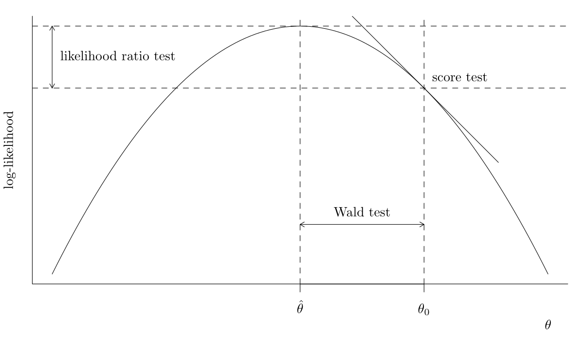
• Therefore, the slope (the score) of the log-likelihood function evaluated at ${\beta }_j=0$ should be close to zero.

Conversely, if the slope at ${\beta }_j=0$ is very steep, it implies that the likelihood would increase significantly if we allowed ${\beta }_j$ to move away from 0. This provides strong evidence against the null hypothesis.

The following video segment explains this graphical intuition beautifully.

This image provides a static view of the same concept, comparing the Score test to the Wald and LRT tests we've already covered.

3. The General Procedure and Key Advantage

The most important feature of the Score test—and its primary advantage—is that it only requires fitting the simpler, restricted model (i.e., the model under the null hypothesis).

Here is the general procedure for testing if a set of parameters is zero:

1. State the Hypotheses:

   • $H_0$: The parameters in question are zero. This defines the restricted model.
   • $H_A$: At least one of the parameters is not zero. This corresponds to the full model.

2. Fit the Restricted Model: Fit the GLM that omits the predictor(s) you are testing. For example, if you are testing if ${\beta }_{\text{math}}$ and ${\beta }_{\text{science}}$ are zero, you would fit the model response ~ other_predictors.

3. Calculate the Test Statistic: This is the crucial step. The Score test statistic is calculated using:

   • The score vector $\mathbf{U}(\mathbf{\beta })$ from the full model's log-likelihood, but evaluated at the parameter estimates from the restricted model.
   • The Fisher information matrix $\mathbf{I}(\mathbf{\beta })$, which is essentially the variance-covariance matrix of the parameters. This is also evaluated at the estimates from the restricted model.

The general form of the multivariate Score statistic is:

where $\tilde{\mathbf{\beta }}$ are the parameter estimates from the restricted (null) model. Under $H_0$, this statistic follows a Chi-square distribution with degrees of freedom equal to the number of parameters being tested.

Don't worry about calculating this by hand. The key takeaway is that every component is calculated using only the results of the simpler, restricted model.

This next reading from UCLA Statistics explains this practical advantage very clearly.

Because you only need to fit the simple model, the Score test is computationally efficient. It's ideal for situations in model selection where you have a simple model and want to quickly test whether adding a large group of new candidate predictors would be worthwhile, without having to fit that complex new model. In R, you can perform a Score test using the anova() function with the argument test = "Rao".

Conclusion

You have now been introduced to the three main pillars of hypothesis testing in GLMs: the Likelihood Ratio, Wald, and Score tests.

Key Takeaways for the Score Test:

• Purpose: The Score test assesses if a set of parameters can be fixed to their null-hypothesized values (usually zero).
• Core Idea: It checks if the slope (score) of the log-likelihood function is significantly different from zero when evaluated at the parameter values specified by the null hypothesis.
• General Procedure: Fit the simpler, restricted model (under $H_0$) and use its estimates to calculate the score and information matrix of the full model.
• Key Advantage: It is computationally efficient because it does not require fitting the full, more complex model. This makes it an excellent "omitted variable" test.

In the final lesson of this module, we will bring everything together. We will compare the properties of the Likelihood Ratio, Wald, and Score tests to give you a clear "when to use which" strategy for your exam.