Chi-Square and Fisher's Exact Test Application

Hello! Welcome to our next lesson.

In the last two lessons, we established a clear decision-making framework. First, you learned how to choose between a contingency table analysis and a GLM. Then, you learned the critical rule for deciding between a chi-square test and Fisher's exact test based on expected cell frequencies.

Now, it's time to put all that knowledge into practice. This lesson is all about application, which is crucial for your exam. We'll walk through a complete problem from start to finish, just as you would need to on the test.

Our learning outcome is to: Solve an application problem requiring a chi-square or Fisher's exact test, from problem setup to final conclusion.

We will cover the full workflow for both tests:

Stating hypotheses.
Calculating expected frequencies and choosing the correct test.
Calculating the test statistic or exact p-value.
Drawing a final, context-based conclusion.

Let's begin with a complete, worked example of the Pearson Chi-Square test.

1. The Chi-Square Test: A Complete Worked Example

When faced with an exam question involving two categorical variables, you should follow a structured, step-by-step process. The following video provides an excellent walkthrough of a chi-square test of independence. We will use it to guide our process.

Test of Independence Using Chi-Square Distribution

This video from The Organic Chemistry Tutor, 'Test of Independence Using Chi-Square Distribution', provides a clear, step-by-step solution to a typical exam-style problem. We will follow its structure to learn the complete workflow.

Please watch the entire video (approximately 13 minutes). I will break down the key steps below to structure your viewing. Pay attention to how each step logically follows the previous one.

Let's organize the content from the video into a clear, algorithmic workflow that you can use on your exam.

Step 1: State the Hypotheses and Prepare the Table (0:00 - 2:00 in video)

The first step is always to understand the research question and formalize it with null and alternative hypotheses.

Research Question: Is the average number of hours students study dependent on the type of student (freshman vs. senior)?
Null Hypothesis (H₀): The two variables are independent. The number of study hours is independent of the student type.
Alternative Hypothesis (Hₐ): The two variables are not independent. The number of study hours is dependent on the student type.

The video then shows how to complete the contingency table by calculating the row and column totals (the marginals). This is a crucial preliminary step.

Step 2: Calculate Expected Frequencies (3:59 - 8:28 in video)

This is the most important step for deciding which test to use. The expected frequency for each cell is calculated under the assumption that H₀ is true (i.e., the variables are independent).

The formula is:

E_{ij} = \frac{( Row _{i} Total ) \times ( Column _{j} Total )}{Grand Total}

The video demonstrates this calculation for all six cells. For example, for the top-left cell (Freshmen, 0-2 hours):

Observed count $O_{11}$ = 76
Expected count $E_{11} = \frac{310 \times 223}{630} \approx 109.7$

Decision Point: At this stage, you must check the assumption we learned in the previous lesson.

Check: Are all expected frequencies ≥ 5?
Analysis: In the video's example, the smallest expected count is calculated to be 76.3. All expected counts are well above 5.
Conclusion: The Pearson Chi-Square test is appropriate.

Step 3: Calculate the Chi-Square Test Statistic (8:28 - 11:47 in video)

Now that we've confirmed the chi-square test is valid, we compute the test statistic, which measures the total discrepancy between the observed (O) and expected (E) counts.

The formula is:

χ^{2} = all cells \sum \frac{( O _{ij} - E _{ij} ) ^{2}}{E _{ij}}

The video walks through this sum, calculating a contribution for each of the six cells and adding them up to get the final test statistic:

χ^{2} \approx 32.3

Step 4: Determine Significance and Draw a Conclusion (11:47 - 13:03 in video)

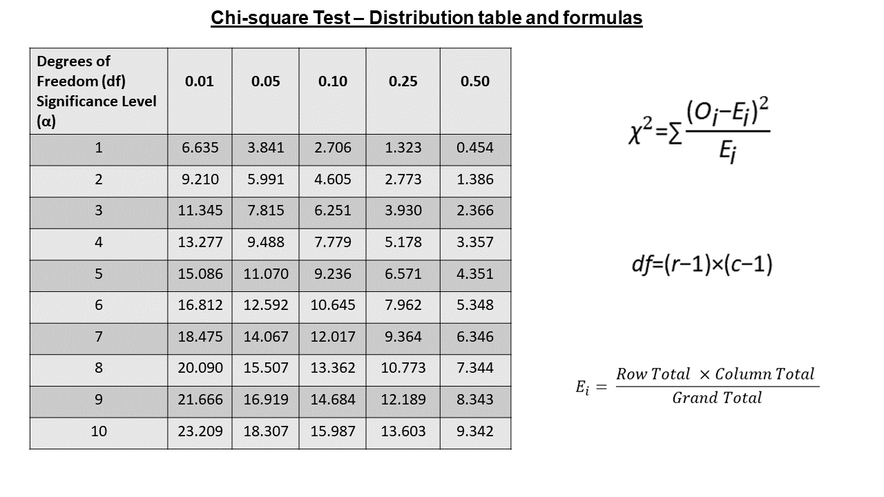
To determine if the calculated $χ^{2}$ value is statistically significant, we compare it to a critical value from the chi-square distribution or, more commonly, we find the corresponding p-value.

Degrees of Freedom (df): This determines the shape of the chi-square distribution we use for comparison. $df = (number of rows - 1) \times (number of columns - 1) = (2 - 1) \times (3 - 1) = 2$
Making a Decision: The video uses the critical value approach. With df=2 and a significance level of $α = 0.05$ , the critical value is 5.99. Since our calculated statistic (32.3) is much larger than the critical value (5.99), it falls into the rejection region.
Conclusion: We reject the null hypothesis. There is statistically significant evidence of an association between the type of student and the average number of hours they study.

Chi-square Test: Distribution Table and Formulas — This image provides a handy reference for the formulas used in a Chi-square test, including the test statistic, degrees of freedom, and expected frequencies. The table shows critical values, which you can use to determine significance, as was done in the video.

2. Fisher's Exact Test: A Complete Worked Example

Now, let's tackle a problem where the chi-square test is not appropriate, forcing us to use Fisher's Exact Test.

Scenario: A veterinary researcher tests whether a rare genetic mutation is associated with a specific disease in a small breed of dogs.

Observed Data:

	Disease Present	Disease Absent	Row Total
Mutation Present	7	2	9
Mutation Absent	3	8	11
Column Total	10	10	20

Let's follow our workflow.

Step 1: State the Hypotheses

H₀: There is no association between the genetic mutation and the disease.
Hₐ: There is an association between the genetic mutation and the disease.

Step 2: Calculate Expected Frequencies and Decide the Test

Let's calculate the expected frequency for the top-left cell (Mutation Present, Disease Present):

E_{11} = \frac{( Row 1 Total ) \times ( Column 1 Total )}{Grand Total} = \frac{9 \times 10}{20} = 4.5

Decision Point: We immediately find an expected frequency (4.5) that is less than 5. We don't need to calculate the rest. The assumption for the chi-square test is violated.
Conclusion: We must use Fisher's Exact Test.

Step 3: Calculate the Exact P-Value

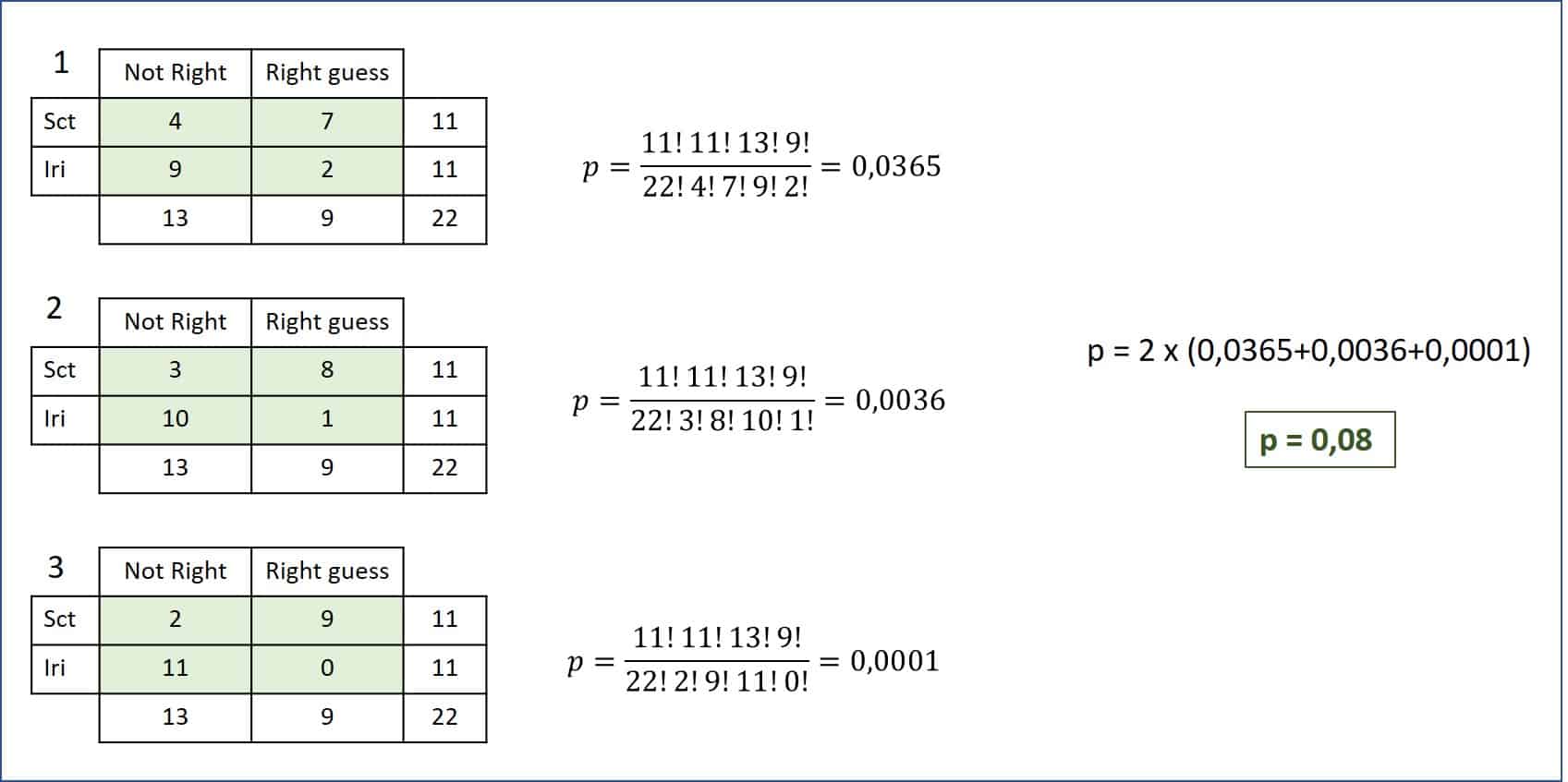
This is where Fisher's test differs significantly from the chi-square test. Instead of an approximate test statistic, we calculate the exact probability of observing our table, and any other tables that are "more extreme," given that the marginal totals are fixed.

The video below explains the logic behind this calculation, which is based on the hypergeometric distribution.

Fisher's test and how to calculate the exact p-value

The video 'Fisher's test and how to calculate the exact p-value' from TileStats explains the core concepts of the test. Focus on how the p-value is built by summing probabilities.

Please watch from 02:10 to 13:00. This is the most important part of the video. Pay close attention to: The analogy of drawing balls from a box to understand the hypergeometric probability (02:10 - 08:32). The concept of finding 'more extreme' tables and summing their probabilities to get the final p-value (08:32 - 13:00).

Let's apply this logic to our dog mutation example.

1. Probability of the Observed Table:
The probability of any given 2x2 table with fixed marginals is given by the hypergeometric probability formula:

P (table) = \frac{( a + b )! ( c + d )! ( a + c )! ( b + d )!}{N ! a ! b ! c ! d !}

For our observed table (a=7, b=2, c=3, d=8):

P (observed) = \frac{9 ! \cdot 11 ! \cdot 10 ! \cdot 10 !}{20 ! \cdot 7 ! \cdot 2 ! \cdot 3 ! \cdot 8 !} = 0.0359

2. Identify and Calculate Probabilities of "More Extreme" Tables:
"More extreme" means an even stronger association in the same direction. In our table, 7 out of 9 dogs with the mutation have the disease. A more extreme table would have 8 or 9 dogs with the mutation having the disease, while keeping the totals fixed.

Extreme Table 1 (a=8):

	Disease Present	Disease Absent	Row Total
Mutation Present	8	1	9
Mutation Absent	2	9	11
Column Total	10	10	20

P (extreme 1) = \frac{9 ! \cdot 11 ! \cdot 10 ! \cdot 10 !}{20 ! \cdot 8 ! \cdot 1 ! \cdot 2 ! \cdot 9 !} = 0.0030

Extreme Table 2 (a=9):

	Disease Present	Disease Absent	Row Total
Mutation Present	9	0	9
Mutation Absent	1	10	11
Column Total	10	10	20

P (extreme 2) = \frac{9 ! \cdot 11 ! \cdot 10 ! \cdot 10 !}{20 ! \cdot 9 ! \cdot 0 ! \cdot 1 ! \cdot 10 !} = 0.00008

(Note: $0! = 1$ )

3. Sum the Probabilities for the P-value:
The one-sided p-value is the sum of probabilities of all tables as extreme or more extreme than what we observed.

p-value (one-sided) = P (observed) + P (extreme 1) + P (extreme 2)

p-value = 0.0359 + 0.0030 + 0.00008 = 0.03898

For a two-sided test, the calculation is more complex, but for your exam, understanding how to construct the one-sided p-value is the key conceptual step. Most software reports a two-sided p-value, which for this data is approximately 0.0498 (as seen in the resource LINK).

Fisher's Exact Test P-value Calculation Example — This image provides a great visualization of what we just did. It shows an observed table and more extreme tables, calculates the probability for each, and sums them to get the final p-value.

Step 4: Draw a Conclusion

Using a significance level of $α = 0.05$ :

Our calculated one-sided p-value is $\approx 0.039$ .
The more standard two-sided p-value is $\approx 0.050$ .
Decision: Since $0.039 < 0.05$ (and $0.050 \approx 0.05$ ), we have evidence to reject the null hypothesis.
Conclusion: We reject H₀. There is a statistically significant association between the genetic mutation and the presence of the disease in this breed of dogs.

3. Final Practice

Now it's your turn. Here is a problem. Follow the workflow we just established to solve it.

Problem: A small software startup wants to know if there is an association between the operating system a developer uses (macOS vs. Windows) and their preference for a new code editor (Editor A vs. Editor B). They survey 25 of their developers.

Observed Data:

	Prefers Editor A	Prefers Editor B	Row Total
macOS	10	2	12
Windows	4	9	13
Column Total	14	11	25

Your Task:

State the null and alternative hypotheses.
Calculate the expected frequencies for all four cells.
Based on the expected frequencies, decide whether to use a Chi-Square test or Fisher's Exact Test.
Perform the chosen test and find the p-value. (If it's Fisher's, you only need to calculate the probability of the observed table to show you understand the process).
State your final conclusion in the context of the problem, using $α = 0.05$ .

Click here to see the solution

1. Hypotheses:

H₀: There is no association between operating system and editor preference.
Hₐ: There is an association between operating system and editor preference.

2. Expected Frequencies:

macOS / Editor A: $E_{11} = (12 \times 14) /25 = 6.72$
macOS / Editor B: $E_{12} = (12 \times 11) /25 = 5.28$
Windows / Editor A: $E_{21} = (13 \times 14) /25 = 7.28$
Windows / Editor B: $E_{22} = (13 \times 11) /25 = 5.72$

3. Decision:
All expected frequencies are greater than 5. Therefore, the Pearson Chi-Square test is appropriate.

4. Perform Test:

Chi-Square Statistic: $χ^{2} = \frac{( 10 - 6.72 ) ^{2}}{6.72} + \frac{( 2 - 5.28 ) ^{2}}{5.28} + \frac{( 4 - 7.28 ) ^{2}}{7.28} + \frac{( 9 - 5.72 ) ^{2}}{5.72}$ $χ^{2} = 1.598 + 2.043 + 1.481 + 1.884 = 7.006$
Degrees of Freedom: $df = (2 - 1) \times (2 - 1) = 1$
P-value: For a $χ^{2}$ value of 7.006 with 1 df, the p-value is approximately 0.008. You would find this using a $χ^{2}$ table or calculator.

5. Conclusion:
Since the p-value (0.008) is less than alpha (0.05), we reject the null hypothesis. There is a statistically significant association between the operating system a developer uses and their preference for the new code editor.

Conclusion

Congratulations! You have now mastered the complete end-to-end process for solving application problems with both the Chi-Square and Fisher's Exact tests. You can confidently identify the correct test and execute it to reach a conclusion.

Key Takeaways:

Always start by stating hypotheses and calculating marginal totals.
The crucial step is to calculate expected frequencies to decide between the Chi-Square test (all E ≥ 5) and Fisher's Exact Test (any E < 5).
For the Chi-Square test, you sum the (O-E)²/E contributions to get the test statistic.
For Fisher's Exact Test, you calculate the exact probability of the observed table and all more extreme tables using the hypergeometric formula.

Preview of the Next Lesson:
We are now moving into the final stage of exam preparation. In the next lesson, you will be presented with a mix of different problem descriptions. Your task will not be to solve them completely, but to practice the rapid-fire skill of correctly identifying the required statistical analysis for each problem, a key skill for efficiently navigating your exam.

Recommended resources