Logistic Regression: From Problem to Interpretation

Hello! Welcome to the final lesson in the "Applied GLM: Logistic Regression" module.

In our last session, we mastered a complete workflow for tackling application problems using chi-square and Fisher's exact tests. You learned how to move from a problem description to a statistical conclusion, a skill that's vital for your exam.

Today, we'll apply that same structured, end-to-end approach to logistic regression. While contingency table tests tell us if an association exists, logistic regression allows us to build a predictive model that explains how multiple predictor variables influence a binary outcome. This is a powerful step up in modeling complexity and a key topic for your midterm.

Our learning outcome is to: Solve an application problem requiring a logistic regression model, from model specification to coefficient interpretation.

By the end of this lesson, you will be able to take a problem with a binary outcome and several predictors, and confidently:

Specify the correct logistic regression model.
Interpret the output from statistical software.
Explain the meaning of the model's intercept and coefficients in terms of odds and odds ratios.
Draw a meaningful conclusion based on the analysis.

Let's get started.

1. The Logistic Regression Workflow: An Overview

When you're faced with a problem that involves predicting a binary outcome (e.g., pass/fail, churn/no-churn, yes/no) from one or more explanatory variables, logistic regression is often the tool of choice.

Why not just use linear regression? Because a linear model can predict probabilities outside the logical 0-to-1 range. Logistic regression solves this by using a sigmoid (S-shaped) curve.

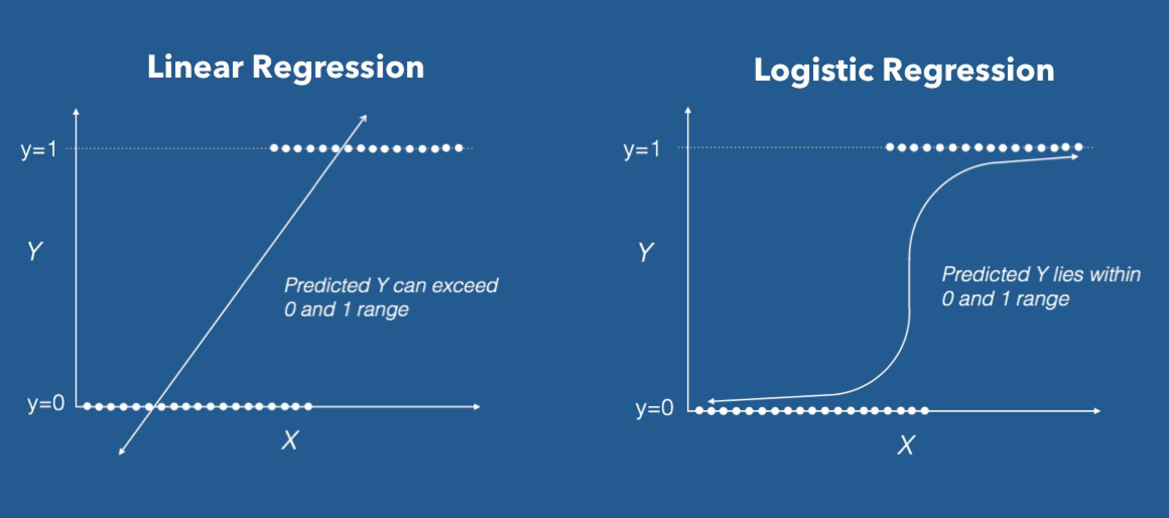
Linear vs. Logistic Regression: Predicted Output Range — This image shows why linear regression is unsuitable for binary outcomes. The straight line predicts values below 0 and above 1, which are impossible for probabilities. The logistic regression curve on the right is constrained between 0 and 1, making it a perfect fit.

Our workflow for a logistic regression problem will be:

Model Specification: Define the problem and write the model equation.
Model Fitting: Understand the software output that provides the estimated coefficients.
Coefficient Interpretation: Explain what the intercept and each predictor's coefficient mean.
Conclusion: Summarize the findings in the context of the original problem.

We'll walk through these steps with a detailed example.

2. A Complete Worked Example: Predicting Honors Admission

Let's use a classic example to illustrate the entire process.

Problem: We want to build a model to understand what factors predict a student's admission into an honors program. Our outcome variable is binary: honors (1 = yes, 0 = no). Our predictor variables are:

female: A binary predictor (1 = female, 0 = male).
math: A continuous predictor representing the student's math score.
read: A continuous predictor representing the student's reading score.

Step 1: Model Specification

Since the outcome is binary and we have multiple predictors, this is a perfect case for logistic regression. The model links the probability of being in the honors program, $P (honors = 1)$ , to a linear combination of the predictors through the logit link function.

The model equation is:

logit (p) = ln (\frac{p}{1 - p}) = β_{0} + β_{1} \cdot female + β_{2} \cdot math + β_{3} \cdot read

Where $p$ is the probability of being admitted to the honors program. Our goal is to find the values of the coefficients ( $β_{0}, β_{1}, β_{2}, β_{3}$ ) that best fit our data.

Step 2: Model Fitting and Understanding the Output

As we discussed in the "Parameter Estimation in GLMs" module, these coefficients are typically estimated using Maximum Likelihood Estimation (MLE), often implemented with an algorithm like Iteratively Reweighted Least Squares (IRWLS). For your exam, you won't need to perform these calculations but you do need to interpret the final output from statistical software.

Here is a typical output for our model:

Predictor	Coefficient ( $β$ )	Std. Error	z-value	p-value	Odds Ratio ( $e^{β}$ )
Intercept	-11.770	1.711	-6.88	< 0.001	0.000
female	0.980	0.422	2.32	0.020	2.664
math	0.123	0.031	3.93	< 0.001	1.131
read	0.059	0.027	2.22	0.026	1.061

Step 3: Coefficient Interpretation

This is the most critical part of the analysis. We need to interpret what each number in the table tells us about the relationship between our predictors and the outcome. The following resources provide excellent, detailed explanations of this process.

FAQ: How do I interpret odds ratios in logistic regression?

First, let's build the core concepts. This FAQ from the UCLA Statistical Consulting Group is a fantastic guide to interpreting logistic regression output. It builds from the ground up, starting with probability and odds, then interpreting coefficients for different types of predictors.

Please read the page from the beginning through the section 'Logistic regression with multiple predictor variables and no interaction terms'. This will take about 15 minutes. Focus on: The transformation from probability to odds to log-odds. How the intercept is the baseline log-odds. How a coefficient represents the change in log-odds. How exponentiating a coefficient gives the odds ratio.

Logistic Regression Details Pt1: Coefficients

For a more visual and intuitive explanation, this StatQuest video is one of the best resources available. It masterfully explains how to think about coefficients for both continuous and discrete predictors.

Please watch from 04:36 to 18:37. Pay close attention to: How the logit transformation straightens the 'S' curve (04:36 - 08:09). The interpretation of the intercept and the slope for a continuous predictor (weight) (08:09 - 10:36). The interpretation of coefficients for a dichotomous predictor (gene mutation), which is exactly like our 'female' variable (10:36 - 18:37).

Now, let's apply the principles from these resources to our honors admission example.

Interpreting the Intercept ( $β_{0} = - 11.770$ )

The intercept is the log-odds of being admitted to the honors program for a student for whom all predictors are zero.
In our case, this means a male student (female=0) with a math score of 0 and a reading score of 0.
The log-odds are $- 11.770$ . The odds are $e^{- 11.770}$ , which is a very tiny number, extremely close to zero. This makes sense—a student with zero scores has almost no chance of getting into an honors program.

Interpreting the female Coefficient ( $β_{1} = 0.980$ )

This is a dichotomous predictor. The coefficient represents the change in log-odds when moving from the reference group (female=0, i.e., males) to the other group (female=1, i.e., females), holding all other variables constant.
Log-odds interpretation: Holding math and reading scores constant, the log-odds of admission for females are 0.980 higher than for males.
Odds Ratio interpretation: The odds ratio is $e^{0.980} = 2.66$ . This means that, holding scores constant, the odds of being admitted for females are 2.66 times the odds for males.
Significance: The p-value is 0.020, which is less than 0.05. This indicates that gender is a statistically significant predictor of admission.

Interpreting the math Coefficient ( $β_{2} = 0.123$ )

This is a continuous predictor. The coefficient represents the change in log-odds for a one-unit increase in the predictor, holding other variables constant.
Log-odds interpretation: For every one-point increase in a student's math score, the log-odds of being admitted to the honors program increase by 0.123, holding gender and reading score constant.
Odds Ratio interpretation: The odds ratio is $e^{0.123} = 1.13$ . This means that for every one-point increase in math score, the odds of admission are multiplied by 1.13 (or increase by 13%), holding other variables constant.
Significance: The p-value is < 0.001, so math score is a highly significant predictor.

Interpreting the read Coefficient ( $β_{3} = 0.059$ )

Similar to math, this is a continuous predictor.
Odds Ratio interpretation: For every one-point increase in reading score, the odds of admission increase by a factor of $e^{0.059} = 1.06$ (a 6% increase), holding gender and math score constant.
Significance: The p-value is 0.026, so reading score is also a statistically significant predictor.

Step 4: Stating the Conclusion

Based on our interpretation, we can now form a conclusion in the context of the original problem.

"The logistic regression model shows that math score, reading score, and gender are all significant predictors of admission to the honors program. Specifically, after controlling for other factors:

The odds of admission increase by 13% for each additional point on the math test.

The odds of admission increase by 6% for each additional point on the reading test.

Female students have 2.66 times the odds of being admitted compared to male students."

This type of detailed, context-specific interpretation is exactly what you should aim for on your exam.

3. Practice Problem

Now it's your turn. Let's analyze a different dataset.

Problem: A telecom company wants to understand customer churn. They have data on former customers and want to model the probability of churn (Churn=1) based on the customer's monthly contract type and their tenure (how long they've been a customer in months).

Here is the output from a logistic regression model:

Binary Logistic Regression Output for Churn Prediction — This image shows the output for a logistic regression model predicting customer churn. Use the 'Estimate' column for the coefficients ($\beta$) and the p-values to check significance. The reference category for 'Contract' is 'Month-to-month'.

Your Task:

Write out the logistic regression model equation.
Interpret the coefficient for Tenure. What is the odds ratio, and what does it mean?
Interpret the coefficient for Contract: One year. What is the odds ratio, and what does it mean in comparison to the reference group?
Based on these predictors, what would you tell the telecom company about what influences customer churn?

Click here to see the solution

1. Model Equation:
Let $p$ be the probability of churn. The model includes Tenure (continuous) and Contract (categorical). Since Contract has three levels (Month-to-month, One year, Two year), it is represented by two dummy variables, with 'Month-to-month' as the reference.

ln (\frac{p}{1 - p}) = β_{0} + β_{1} \cdot Tenure + β_{2} \cdot Contract_{One year} + β_{3} \cdot Contract_{Two year}

2. Interpretation of Tenure:

Coefficient ( $β_{1}$ ): From the table, the coefficient for Tenure is -0.035.
Log-odds interpretation: For each additional month a customer stays with the company, the log-odds of them churning decreases by 0.035, holding contract type constant.
Odds Ratio: The odds ratio is $e^{- 0.035} \approx 0.966$ .
Meaning: For each additional month of tenure, the odds of churning are multiplied by 0.966, which means the odds decrease by about 3.4% (since $1 - 0.966 = 0.034$ ). This is highly significant (p < 0.001).

3. Interpretation of Contract: One year:

Coefficient ( $β_{2}$ ): From the table, the coefficient is -1.74.
Log-odds interpretation: The log-odds of churning for a customer with a 'One year' contract are 1.74 lower than for a customer with a 'Month-to-month' contract, holding tenure constant.
Odds Ratio: The odds ratio is $e^{- 1.74} \approx 0.175$ .
Meaning: The odds of churning for a customer on a 'One year' contract are only 0.175 times the odds of churning for a customer on a 'Month-to-month' contract. In other words, the odds of churning are about 82.5% lower for one-year contract holders compared to month-to-month holders. This is also highly significant (p < 0.001).

4. Conclusion for the Company:
"Our analysis indicates that both customer tenure and contract type are extremely strong predictors of churn.

Longer-term customers are significantly less likely to churn; for every additional month a customer stays, their odds of churning decrease by about 3.4%.
Customers on longer contracts are also much less likely to churn. Compared to those on a month-to-month plan, customers on a one-year contract have 82.5% lower odds of churning, and those on a two-year contract have over 95% lower odds of churning.
Efforts to increase customer tenure and encourage switching from monthly to yearly contracts would be effective strategies for reducing churn."

Conclusion

Excellent work! You have now walked through the entire process of solving an application-based logistic regression problem, from specifying the model to interpreting the coefficients and drawing a meaningful conclusion.

Key Takeaways:

Logistic regression models the log-odds of an outcome as a linear function of predictors.
The intercept ( $β_{0}$ ) is the log-odds when all predictors are zero.
A coefficient ( $β_{j}$ ) represents the change in log-odds for a one-unit change in the predictor $x_{j}$ , holding all other predictors constant.
The odds ratio ( $e^{β_{j}}$ ) is the multiplicative factor by which the odds change for a one-unit change in the predictor $x_{j}$ .
Always state your final interpretation in the practical context of the problem.

Preview of the Next Lesson:
You've now developed workflows for both contingency table analysis and logistic regression. In our final lesson, we will focus on exam strategy. You will be given a series of mixed problem descriptions and your only task will be to identify the correct statistical method for each. This will sharpen the critical decision-making skills you need to succeed on your exam.

Recommended resources