Welcome back! In our previous lesson, we explored the concept of time-space tradeoffs, establishing that you can often improve an algorithm's speed by using more memory, or vice-versa. To effectively discuss these tradeoffs, we need a standard language to describe performance.
This lesson concludes our first module on complexity analysis by focusing on that very language. Our goal is to recognize common complexity classes: O(1), O(log n), O(n), O(n log n), O(n²), and O(2^n). Mastering this will allow you to quickly analyze code, predict its performance bottlenecks, and communicate your findings effectively in a technical interview.
The Big Picture: Visualizing Growth Rates
Before diving into each class, let's get a visual intuition for how they compare. The rate at which an algorithm's runtime or space usage grows with the input size is the most important takeaway.
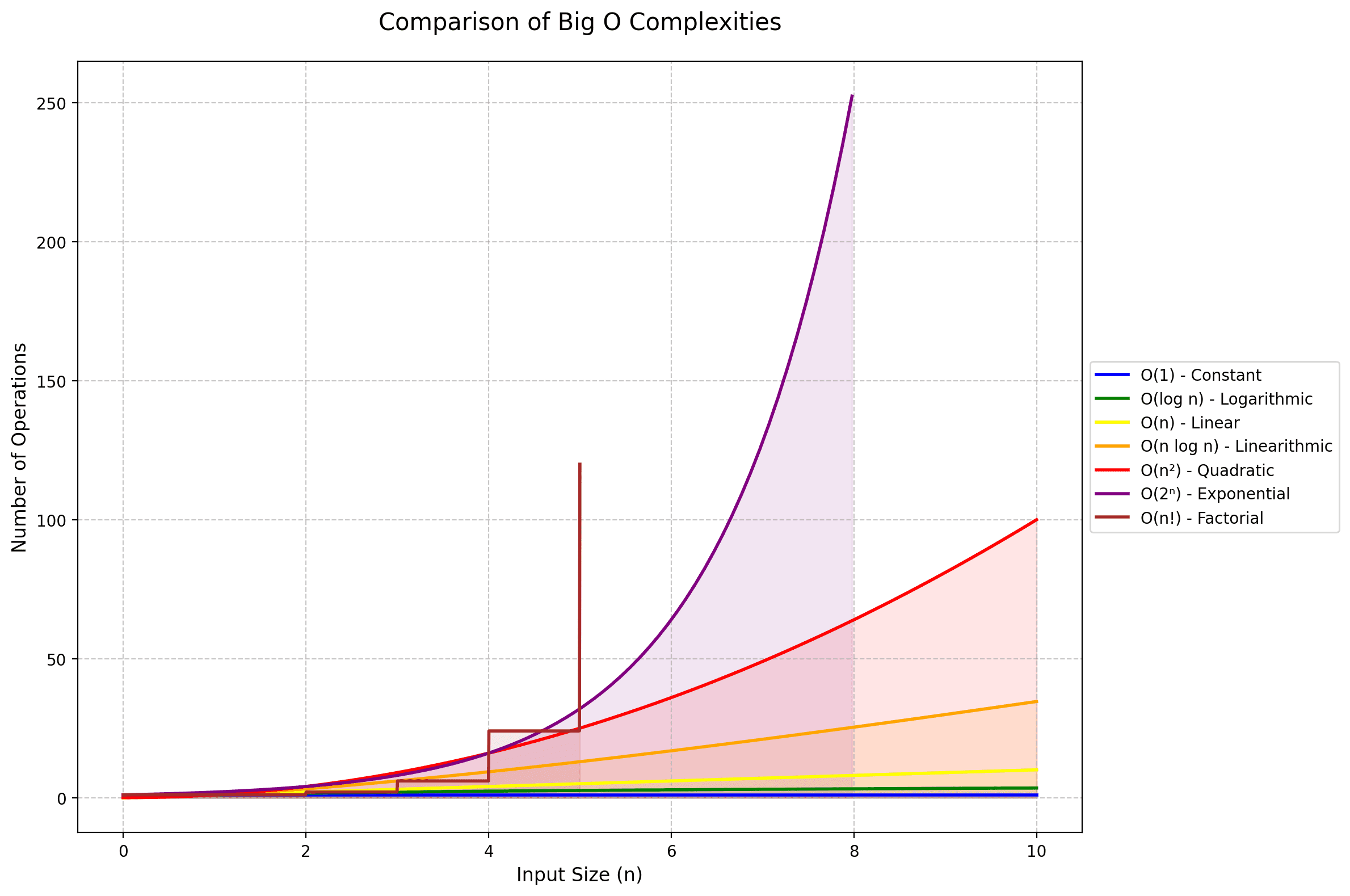
As you can see, the difference between an efficient and an inefficient algorithm is not minor—it's dramatic. Let's break down what each of these curves represents.
A Tour of Common Complexity Classes
We'll now go through the most common complexity classes you'll encounter, from the most efficient to the least. We will use a comprehensive video from NeetCode, a great resource for interview preparation, as our guide.
Big-O Notation - For Coding Interviews
The video 'Big-O Notation - For Coding Interviews' by NeetCode provides a fantastic, interview-focused overview of these concepts. We'll watch it in segments.
We will be watching specific sections of this video throughout the lesson. For now, you don't need to watch anything; just have it ready.
1. O(1) — Constant Time
An algorithm runs in constant time if its execution time is independent of the input size. It takes the same amount of time for 10 elements as it does for 10 million.
- Common Patterns: Direct lookups, simple arithmetic.
- Examples:
- Accessing an element in an array by its index (
my_array[5]). - Pushing or popping from a stack.
- Inserting or looking up a value in a hash map (on average).
- Accessing an element in an array by its index (
Big-O Notation - For Coding Interviews
Let's start with the fastest complexity class. Watch this segment from the NeetCode video to see examples of O(1) operations.
Watch from 01:51 to 02:53. The video explains why operations that don't depend on the input size are considered constant time.
2. O(log n) — Logarithmic Time
Logarithmic time complexity is incredibly efficient. These algorithms work by repeatedly cutting the problem size, typically by a constant factor (like one-half) at each step. If you double the input size, you only add one extra "step" to the process.
- Common Patterns: Divide and conquer algorithms that discard a large portion of the input at each step.
- Examples:
- Binary search in a sorted array.
- Finding an element in a balanced Binary Search Tree (BST).
- Pushing to or popping from a heap/priority queue.
Logarithms can be tricky. Let's watch two videos to solidify this concept. The first is from NeetCode, and the second provides a more focused, visual explanation.
Big-O Notation - For Coding Interviews
First, let's see how NeetCode explains O(log n) in the context of binary search.
Watch from 10:49 to 13:18. Pay attention to the core idea: how many times can you divide n by 2 until you get to 1? That's the essence of log base 2.
Big O Notation Series #4: The Secret to Understanding O (log n)!
For a more detailed breakdown, this video 'The Secret to Understanding O (log n)!' from Kantan Coding is excellent.
Watch from 00:20 to 04:41. It visualizes how dividing a number (e.g., 8) by 2 repeatedly directly corresponds to the number of steps, which is log₂(8) = 3.
3. O(n) — Linear Time
This is a very common and generally good complexity. The runtime grows linearly with the size of the input. If the input size doubles, the runtime also roughly doubles.
- Common Patterns: A single loop that iterates through all
nelements of a collection. - Examples:
- Iterating through an array or linked list.
- Finding the minimum or maximum element in an unsorted array.
- Linear search (checking every element for a target).
Big-O Notation - For Coding Interviews
Now for linear time. Let's return to the NeetCode video.
Watch from 02:53 to 05:56. This segment covers various scenarios that result in O(n) complexity, including looping and, importantly, insertion/deletion in the middle of an array (which requires shifting elements).
Test your understanding!
Consider a function that takes two separate lists, list_a of size n and list_b of size m, as input. The function iterates through list_a once, and then it iterates through list_b once. What is the time complexity?
Show answer
The time complexity is O(n + m).
Since the loops are separate (not nested), their runtimes add up. The first loop takes O(n) time, and the second takes O(m) time. In Big O analysis, if n and m represent different input sizes that can vary independently, you must keep both terms. You cannot simplify this to O(n) or O(m).
4. O(n log n) — Linearithmic Time
This complexity class is often seen in efficient sorting algorithms. It's better than quadratic but worse than linear. You can think of it as doing a logarithmic amount of work for each of the n items.
- Common Patterns: Divide and conquer algorithms where the work is split and then merged back together.
- Examples:
- Merge Sort and Heap Sort.
- The average case for Quicksort.
Big-O Notation - For Coding Interviews
Let's see where O(n log n) comes from. This segment of the NeetCode video explains it in the context of sorting.
Watch from 13:18 to 15:02. The explanation of Heap Sort is a great example: you perform n pop operations, and each pop from the heap takes O(log n) time, resulting in O(n log n).
5. O(n²) — Quadratic Time
Quadratic time complexity often appears when you have to compare every element in a collection to every other element. As the input size grows, the runtime grows much faster. Doubling the input size quadruples the runtime.
- Common Patterns: Nested loops over the same input collection.
- Examples:
- Simple sorting algorithms like Bubble Sort, Selection Sort, and Insertion Sort.
- Finding all pairs of elements in a list.
Big-O Notation - For Coding Interviews
Nested loops are the classic sign of quadratic complexity. Let's see how NeetCode breaks this down.
Watch from 06:37 to 09:34. The video provides an excellent visual for why a nested loop where the inner loop's range decreases (for i in n: for j in i: ...) still results in O(n²) complexity (the triangle is half a square).
6. O(2ⁿ) — Exponential Time
Exponential time algorithms are very slow and become impractical for all but the smallest input sizes. Each additional element in the input roughly doubles the runtime.
- Common Patterns: Recursive algorithms that solve a problem of size
nby recursively solving two or more subproblems of sizen-1. - Examples:
- The recursive calculation of Fibonacci numbers (without memoization).
- Generating all subsets of a set (the power set).
Big-O Notation - For Coding Interviews
Finally, let's look at exponential time. These are the algorithms you generally want to avoid if a more efficient alternative exists.
Watch from 15:02 to 16:01. This segment shows how a recursive function with two branches for each call can lead to an O(2ⁿ) runtime.
Quick Reference and Summary
To tie everything together, here is a summary table. Being able to quickly recall common examples for each complexity class is a valuable skill for interviews.
Big O Complexity Cheat Sheet for Coding Interviews
The article 'Big O Complexity Cheat Sheet for Coding Interviews' from KDnuggets offers a concise summary table that is perfect for review.
Focus on the 'Big-O Complexity Reference Table'. It neatly summarizes the name, description, and common use cases for each complexity we've discussed, plus O(n!) (factorial), which is even slower than exponential.
Here's that information presented as a Markdown table for your convenience:
| Complexity | Name | Description | Common Use Cases | Performance at Scale |
|---|---|---|---|---|
| O(1) | Constant | Runtime unaffected by input size | Hash tables, array access | Excellent |
| O(log n) | Logarithmic | Runtime increases slowly | Binary search, balanced trees | Very good |
| O(n) | Linear | Runtime scales linearly | Linear search, array traversal | Good |
| O(n log n) | Linearithmic | Between linear and quadratic | Efficient sorting algorithms | Fair |
| O(n²) | Quadratic | Runtime squares with input size | Nested loops, simple sorting | Poor |
| O(2ⁿ) | Exponential | Runtime doubles with each input | Recursive solutions, combinatorics | Very poor |
| O(n!) | Factorial | Runtime grows by factorial | Permutations, traveling salesman | Terrible |
Conclusion
This lesson concludes our foundational module on complexity analysis. You can now calculate time and space complexity, analyze tradeoffs, and recognize the common complexity classes that define algorithmic performance.
Key Takeaways:
- Growth Rate is Key: Big O notation describes how an algorithm's resource usage scales with input size.
- Pattern Recognition: Specific code structures reliably lead to certain complexities (e.g., nested loops -> O(n²), divide-and-halve -> O(log n)).
- The Hierarchy of Efficiency:
O(1) < O(log n) < O(n) < O(n log n) < O(n²) < O(2ⁿ) < O(n!). Knowing this hierarchy helps you quickly judge whether an algorithm is efficient.
With this analytical framework in place, you are now ready to apply it to concrete data structures. In our next lesson, we will begin Module 2: Core Sequential Data Structures by diving into the implementation and analysis of dynamic arrays.