Dynamic Array Operations

Hello! Welcome to the second module of our course. In the last lesson, we built a strong foundation by identifying the common complexity classes like $O (1)$ , $O (n)$ , and $O (lo g n)$ . This vocabulary is essential for analyzing and discussing algorithms, which is a core skill for technical interviews.

Today, we transition from theory to practice. We will implement and analyze one of the most fundamental and frequently used data structures: the dynamic array. Your goal for this lesson is to be able to implement and analyze the core operations of a dynamic array (often called a vector or ArrayList in different languages). We'll see how the complexities we just learned, especially the idea of an "average" or amortized cost, play out in a real-world data structure.

From Static to Dynamic: The Need for Flexibility

Standard arrays are powerful because they offer constant-time, $O (1)$ , access to any element via its index. However, they have a major limitation: their size is fixed upon creation. If you need to store more elements than you initially planned for, you're out of luck.

This is where dynamic arrays come in. They provide the flexibility of a list that can grow or shrink on demand, while still trying to maintain the performance benefits of a standard array.

Let's start with a quick overview of their main characteristics.

Dynamic Array Data Structure

The article 'Dynamic Array Data Structure' from Interview Cake gives a concise summary of the strengths and weaknesses of this data structure. It's a great starting point.

Please read the introduction and the 'Strengths' and 'Weaknesses' sections. This will give you a high-level picture before we dive into the implementation details.

As you've read, the key trade-off is that while appends are usually fast, they can sometimes be slow. Let's dissect how this works by building a dynamic array from scratch.

Building a Dynamic Array

We will use Python for our implementation, leveraging your familiarity with the language. The core idea is to use a regular, fixed-size array (in Python, this can be simulated with a list of a pre-allocated size) under the hood and manage its capacity ourselves.

The following video provides an excellent, step-by-step walkthrough of creating a DynamicArray class.

Design a Dynamic Array (Resizable Array)

The video 'Design a Dynamic Array (Resizable Array)' by NeetCode is a practical guide that aligns perfectly with our learning outcome. We'll go through its implementation and analysis in stages.

We will reference different parts of this video throughout the lesson. For now, you can get ready to watch the first segment.

1. Initialization and Basic Operations

First, we need to initialize our array. A dynamic array needs to keep track of two key properties:

Capacity: The size of the underlying fixed-size array.
Size (or length): The number of elements currently stored in the dynamic array.

Naturally, size <= capacity.

Design a Dynamic Array (Resizable Array)

Let's watch how to set up the constructor and implement basic get and set methods.

Watch from 00:33 to 03:11. Notice how the implementation clearly distinguishes between capacity (the length of the internal array) and size (the number of elements the user has added).

The operations covered so far are straightforward:

__init__(capacity): Allocates the internal array. This takes $O (capacity)$ time.
get(i) and set(i, n): Access or modify an element at a given index. These are just wrappers around the underlying array's access, so they are $O (1)$ .

2. Appending and the Magic of Resizing

The most critical operation is adding an element to the end of the array, often called append or push_back. This is where the "dynamic" nature comes into play.

The logic is:

Check if size == capacity.
If it is, we are out of space. We must resize the underlying array.
Add the new element at index size.
Increment size.

The resize step is the most interesting part. The standard strategy is to double the capacity of the underlying array. This involves:

Creating a new array with twice the capacity.
Copying all elements from the old array to the new one.
Replacing the old array with the new one.

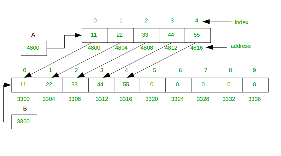
Dynamic Array Resizing and Memory Reallocation — This image illustrates the resizing process. When the original array (A) becomes full, a new, larger array (B) is allocated in a different memory location, and all elements from A are copied over to B.

Let's watch this process in action.

Design a Dynamic Array (Resizable Array)

This part of the NeetCode video implements the push_back method, including the crucial resize logic.

Watch from 03:11 to 06:57. Pay close attention to the resize function. Understand that this copying operation is not free—it takes time proportional to the number of elements being copied.

This copying step is an $O (n)$ operation, where $n$ is the current size of the array. This seems expensive! If push_back can be $O (n)$ , how can we say it's efficient? This brings us to amortized analysis.

Amortized Time Complexity: The Average Cost

While a single push_back operation can be $O (n)$ in the worst case (when a resize is triggered), these expensive operations are infrequent. Most of the time, push_back is a simple $O (1)$ operation.

Amortized analysis averages the cost of these expensive operations over the entire sequence of operations. Because we double the capacity each time, the number of $O (1)$ appends we can do before the next expensive $O (n)$ resize grows exponentially. This "cancels out" the cost of the resize over time.

The result is that the amortized time complexity of push_back is $O (1)$ . This is a critical concept for interviews.

The Simple and Elegant Idea behind Efficient Dynamic Arrays

For a deeper, more intuitive understanding of why doubling leads to O(1) amortized time, this video from Reducible is fantastic. It uses a geometric argument that makes the concept very clear.

Watch from 01:06 to 05:47. The key insight is that the total work to insert n elements (including all resizing costs) is a geometric series that sums to approximately 2n. Therefore, the average work per insertion is O(1).

Test your understanding!

Imagine you're designing a dynamic array, but instead of doubling the capacity upon resize, you decide to just add a fixed constant, say 10 spots, each time (new_capacity = old_capacity + 10). How would this affect the amortized time complexity of appending n elements in a row?

Show answer

The amortized time complexity would become $O (n)$ per operation, which is much worse.

Here's why: To add $n$ elements, you will need to resize roughly $n /10$ times. The costs of these resizes would be approximately 10, 20, 30, ..., $n$ . This is an arithmetic series. The sum of the work done for resizing would be proportional to $10 + 20 + ... + n$ , which is $O (n^{2})$ .

Since the total work to add $n$ elements is $O (n^{2})$ , the amortized cost per append operation becomes $O (n^{2}) / n = O (n)$ . The multiplicative growth (doubling) is essential for achieving $O (1)$ amortized time.

Other Operations and Final Analysis

Now let's round out our implementation and summarize the performance.

pop_back (Remove from end): This is a simple $O (1)$ operation. We just decrement the size variable. We don't need to actually erase the data; it will be overwritten by a future push_back. This is sometimes called a "soft deletion."
insert(i, n) / delete(i) (Middle Operations): This is the dynamic array's main weakness. To insert or delete an element in the middle, you must shift all subsequent elements to the right or left. This is an $O (n)$ operation in the worst case (inserting at the beginning).

Let's watch the final analysis from the NeetCode video.

Design a Dynamic Array (Resizable Array)

This last segment covers pop_back and provides a full time complexity analysis of all the methods we've built.

Watch from 06:57 to 11:16. This will summarize the complexities and confirm your understanding.

Summary of Dynamic Array Operations

Here is a quick reference table for the time complexities of dynamic array operations. This is exactly the kind of knowledge you need to have ready for an interview.

Operation	Time Complexity (Worst Case)	Time Complexity (Amortized)	Notes
Access (`get`)	$O (1)$	$O (1)$	Direct memory access via index.
Modify (`set`)	$O (1)$	$O (1)$	Direct memory access via index.
Append (`push_back`)	$O (n)$	$O (1)$	The $O (n)$ case occurs during a resize.
Pop from End (`pop_back`)	$O (1)$	$O (1)$	Simply decrements the size pointer.
Insert at Index `i`	$O (n)$	$O (n)$	Requires shifting $n - i$ elements.
Delete at Index `i`	$O (n)$	$O (n)$	Requires shifting $n - i - 1$ elements.

Conclusion

In this lesson, you learned how to implement a dynamic array and, more importantly, how to analyze its performance. You saw a real-world application of Big O notation and were introduced to the crucial concept of amortized analysis.

Key Takeaways:

Dynamic arrays solve the fixed-size limitation of static arrays by using an internal, resizable array.
The key to efficiency is the resizing strategy. Doubling the capacity ensures that expensive $O (n)$ resizes are infrequent enough to yield an $O (1)$ amortized time complexity for appends.
Dynamic arrays excel at fast lookups ( $O (1)$ ) and appends ( $O (1)$ amortized), but struggle with insertions and deletions in the middle ( $O (n)$ ).

This final point sets the stage for our next lesson. We've seen that array-based structures are slow for middle insertions/deletions. Next time, we'll explore the singly linked list, a data structure designed to optimize for exactly that, at the cost of slow lookups. This will be our first look at a major data structure tradeoff.

Recommended resources

From Static to Dynamic: The Need for Flexibility

Building a Dynamic Array

1. Initialization and Basic Operations

2. Appending and the Magic of Resizing

Amortized Time Complexity: The Average Cost

Other Operations and Final Analysis

Summary of Dynamic Array Operations

Conclusion