Ridge and Lasso Regularization: Preventing Overfitting and Feature Selection

Welcome to the first lesson in our module on regularized linear models. In our previous lesson, we explored how to interpret the coefficients of a linear regression model. We saw that while these coefficients offer powerful insights, they can become unstable and unreliable in the presence of highly correlated features—a problem known as multicollinearity. We also touched upon the broader challenge of overfitting, where a model learns the training data so well that it fails to generalize to new, unseen data.

This lesson directly addresses these challenges. We will introduce regularization, a fundamental technique in machine learning for creating simpler, more robust models. Specifically, we will dive into two of the most important regularization methods: Ridge (L2) regularization and Lasso (L1) regularization. By the end of this lesson, you will understand the intuition behind each method, how they modify the model's learning process to combat overfitting, and the crucial difference that gives Lasso its celebrated feature selection capability.

The Problem with Complexity and the Idea of a Penalty

In linear regression, our goal is to find the coefficients ( $β$ ) that minimize the sum of squared errors (or Mean Squared Error, MSE). This works well when we have a clean, simple relationship between features and the target. However, with many features, especially correlated or irrelevant ones, the model can "overfit" by assigning extremely large positive and negative coefficient values that contort the regression line to fit noise in the training data. The resulting model is overly complex and performs poorly on new data.

Regularization offers a clever solution: it modifies the cost function to penalize complexity. Instead of only minimizing the error, we now minimize a combination of error and a penalty for large coefficient values.

The new cost function looks like this:

New Cost = Original Cost (e.g., MSE) + Penalty Term

This forces the model into a trade-off: it must find coefficients that fit the data well without letting them become too large. The strength of this penalty is controlled by a hyperparameter, typically denoted by lambda ( $λ$ ) or alpha ( $α$ ). A larger $λ$ imposes a stronger penalty, forcing the coefficients to be smaller.

The "codebasics" video provides a great high-level introduction to this concept.

Machine Learning Tutorial Python - 17: L1 and L2 Regularization | Lasso, Ridge Regression

This video from the "codebasics" channel introduces overfitting and then provides a clear, step-by-step explanation of how adding a penalty term to the MSE function helps control model complexity.

Please watch the following segments: Overfitting example: This gives a quick visual intuition for underfitting, overfitting, and a balanced fit. L2 and L1 Intuition: This is the core part. Pay close attention to how the speaker adds a penalty term (\lambda \times \sum \theta^2 for L2 and \lambda \times \sum |\theta| for L1) to the MSE function. The key takeaway is that this new term penalizes the model for having large coefficients.

The difference between Ridge and Lasso lies entirely in how that penalty is calculated.

Ridge Regression (L2 Regularization)

Ridge regression uses the L2 norm as its penalty. This is the sum of the squared values of all the model's coefficients.

The Ridge cost function is:

Cost_{Ridge} = i = 1 \sum n (y_{i} - y^_{i})^{2} + λ j = 1 \sum p β_{j}^{2}

Here, $β_{j}$ represents each coefficient, and $λ$ controls the penalty strength.

Because the penalty is squared, it has a more pronounced effect on larger coefficients. A coefficient of 10 incurs 100 times more penalty than a coefficient of 1. This encourages the model to shrink all coefficients towards zero, but it very rarely forces them to be exactly zero. Ridge regression is excellent at handling multicollinearity; instead of picking one feature from a group of correlated features and giving it a large coefficient, it tends to distribute the weight more evenly among them, resulting in smaller, more stable coefficients for the whole group.

The following article provides a clear, mathematical explanation of Ridge regression.

Regularization in Machine Learning: Ridge, Lasso, and Elasti

This guide from "letsdatascience.com" offers a comprehensive technical breakdown of regularization. We'll focus on the section about Ridge.

Please read the section titled Ridge regression. Focus on: The cost function formula with the L2 penalty. The "In Plain English" explanation of how the squared penalty punishes large coefficients. The point about how Ridge stabilizes the model in the presence of correlated features.

The StatQuest channel has a fantastic video that visualizes this shrinking effect.

Ridge vs Lasso Regression, Visualized!!!

This video from "StatQuest with Josh Starmer" provides an excellent visual intuition for how the Ridge penalty works.

Watch the segment from the start of the Ridge explanation to the end of the summary. Notice how as the lambda value increases, the parabola representing the cost shifts, and its minimum point (the optimal coefficient) gets closer and closer to zero, but never actually lands on it.

Lasso Regression (L1 Regularization)

Lasso (Least Absolute Shrinkage and Selection Operator) regression uses the L1 norm as its penalty. This is the sum of the absolute values of the coefficients.

The Lasso cost function is:

Cost_{Lasso} = i = 1 \sum n (y_{i} - y^_{i})^{2} + λ j = 1 \sum p ∣ β_{j} ∣

This seemingly small change—using absolute values instead of squared values—has a profound consequence. The L1 penalty applies a constant "tax" on every coefficient, regardless of its size. For small coefficients, this constant pressure is enough to push them all the way to zero.

This means Lasso performs automatic feature selection. By setting the coefficients of irrelevant or redundant features to exactly zero, it effectively removes them from the model, leading to a "sparse" model that is often simpler and more interpretable.

Regularization in Machine Learning: Ridge, Lasso, and Elasti

Now, let's return to the "letsdatascience.com" guide to understand Lasso.

Read the section Lasso regression. Pay attention to: The cost function with the L1 penalty. The "In Plain English" explanation of the linear penalty. The key takeaway: Lasso performs automatic feature selection by setting some coefficients to exactly 0.0.

The StatQuest video again provides the perfect visual for this.

Ridge vs Lasso Regression, Visualized!!!

Let's see the visual comparison of Lasso to Ridge.

Watch the remainder of the video, from the start of the Lasso explanation to the end. The crucial part is the "kink" that forms at zero in the cost curve. This kink makes it possible for the minimum point (the optimal coefficient) to land exactly at zero, effectively eliminating that feature.

The Geometric Interpretation: Circle vs. Diamond

The most elegant way to understand the difference between Ridge and Lasso is to view them as constrained optimization problems. We are trying to find the coefficients ( $β$ ) that minimize the error (the center of the contour plot below), subject to a constraint on the size of the coefficients.

Ridge (L2): The constraint is $\sum β_{j}^{2} \leq C$ . For two coefficients, this forms a circle.
Lasso (L1): The constraint is $\sum ∣ β_{j} ∣ \leq C$ . For two coefficients, this forms a diamond.

The solution is the first point where the expanding elliptical contours of the error function "touch" the constraint boundary.

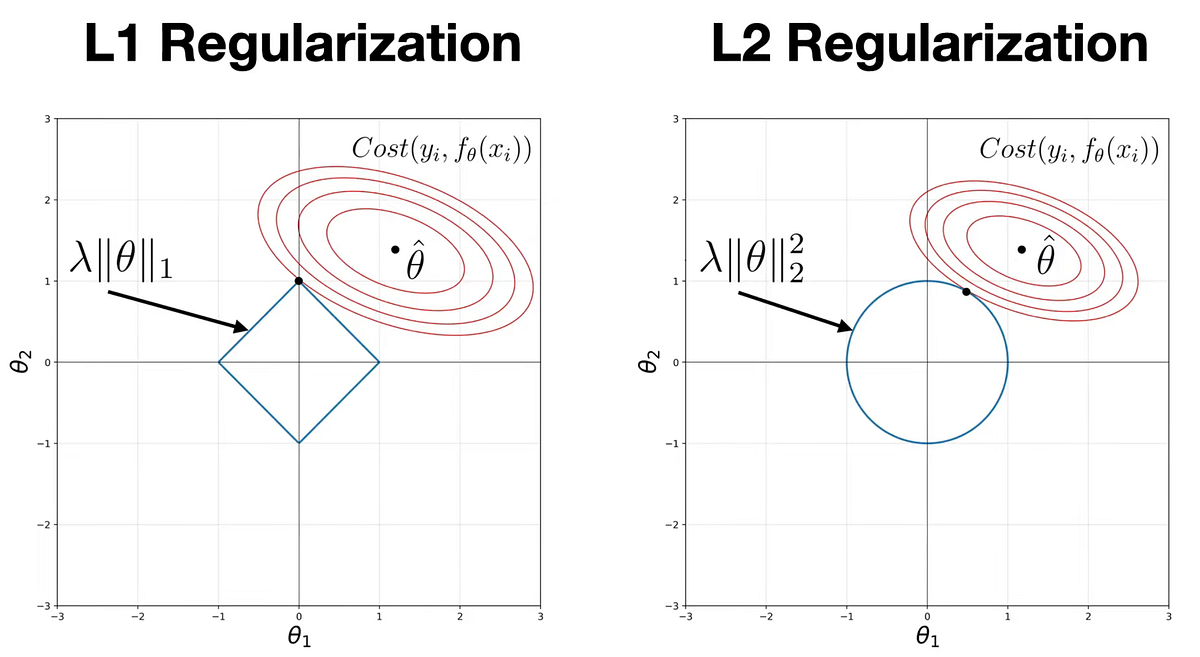
Geometric interpretation of L1 (Lasso) and L2 (Ridge) regularization. The red ellipses are contours of the cost function (e.g., MSE), with the minimum at the center ($\hat{\theta}$). The blue shapes are the constraint regions for the coefficients. The optimal regularized solution is the point of tangency. For L1, this is likely to be at a corner (where a coefficient is zero), while for L2, it can be anywhere on the circle's circumference.

As the image shows, the circular boundary of Ridge has no sharp corners. The error contour is likely to touch it at a point where neither coefficient ( $θ_{1}, θ_{2}$ ) is zero. In contrast, the diamond boundary of Lasso has sharp corners that lie on the axes. It is much more probable that the error contour will make first contact at one of these corners, where one of the coefficients is exactly zero. This is the geometric reason why Lasso performs feature selection and Ridge does not.

For a final reinforcement of these concepts, the following article provides a concise side-by-side comparison.

Understanding L1 and L2 regularization: techniques for ...

This article from Weights & Biases gives a clear comparative summary.

Read the section titled Comparing L1 and L2 Regularization. This section neatly contrasts the two methods on key aspects like handling multicollinearity and model interpretability.

Conclusion

In this lesson, you've explored the fundamental principles of regularization and the two cornerstone techniques, Ridge and Lasso. We've moved from the problem of overfitting and unstable coefficients to a robust solution that improves model generalization.

Key Takeaways:

Regularization prevents overfitting by adding a penalty term to the cost function, discouraging overly complex models with large coefficients.
Ridge (L2) Regression uses a squared penalty ( $λ \sum β_{j}^{2}$ ). It shrinks coefficients towards zero but rarely makes them exactly zero. It's effective at managing multicollinearity by distributing influence among correlated features.
Lasso (L1) Regression uses an absolute value penalty ( $λ \sum ∣ β_{j} ∣$ ). It can shrink coefficients all the way to zero, thus performing automatic feature selection and creating sparse models.
The geometric difference—a circular (L2) vs. a diamond-shaped (L1) constraint—is the intuitive reason behind their different behaviors regarding feature selection.

While Lasso is great for feature selection, it can be unstable when dealing with highly correlated features (it tends to arbitrarily pick one and zero out the others). Ridge is more stable in this scenario but keeps all features. What if we want the best of both worlds?

In our next lesson, we will explore Elastic Net, a hybrid approach that combines the L1 and L2 penalties. We will then transition from theory to practice, applying Ridge, Lasso, and Elastic Net to a real-world dataset using Python and scikit-learn to see their effects on model coefficients and performance firsthand.

Recommended resources

The Problem with Complexity and the Idea of a Penalty

Ridge Regression (L2 Regularization)

Lasso Regression (L1 Regularization)

The Geometric Interpretation: Circle vs. Diamond

Conclusion