In the last lesson, we put theory into practice by building and evaluating a linear regression model from scratch. You saw how to assess a model's predictive power using metrics like R-squared and by visually inspecting its residuals. Now that we know how to measure how well a model predicts, we will turn our attention to understanding how it makes those predictions.
This lesson focuses on interpreting the coefficients of a trained linear regression model. Unlocking the meaning of these values is what elevates a model from a black-box predictor to an explanatory tool. You'll learn how to dissect the model's learned equation to understand the relationship between each feature and the target variable, a crucial step toward your goal of understanding the "why" behind the algorithms.
The Anatomy of a Linear Model
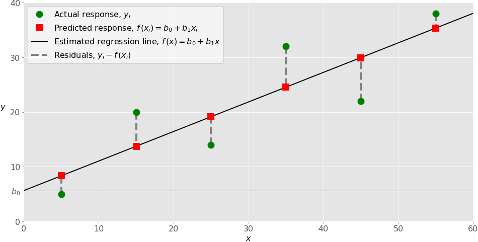
At its heart, a linear regression model is a simple equation. For a model with one feature (simple linear regression), the equation is:
- is the intercept: the predicted value of the target when the feature has a value of zero.
- is the coefficient for the feature: it tells us how much the predicted target is expected to change for a one-unit increase in the feature.
Let's see this in action. The following short video provides a very clear, practical demonstration of how to access these values from a trained scikit-learn model and what they mean.
Hands-On Linear Regression with Scikit-Learn in Python (Beginner Friendly)
This clip from "Hands-On Linear Regression with Scikit-Learn" by Ryan & Matt Data Science gets straight to the point of finding and interpreting the intercept and coefficient.
Watch the segment from extracting coefficients to the intercept explanation. The example predicts salary from years of experience. Pay close attention to how the speaker explains the meaning of the coefficient (the effect of one additional year of experience) and the intercept (the starting salary with zero years of experience).
This simple interpretation is the foundation. Now, let's ground this with another example using a real dataset.
Interpreting Coefficients in Linear Regression Models
This article from Machine Learning Mastery provides excellent, code-driven examples. We'll return to it a few times in this lesson.
For now, read the first section, "Interpreting Coefficients in Linear Models with a Single Numerical Feature." It builds a model to predict house SalePrice from GrLivArea (living area). Notice how the author interprets the coefficient: for each one-unit (square foot) increase in GrLivArea, the price is expected to increase by about $110.
Multiple Regression: The "All Else Being Equal" Principle
Things get more interesting—and more realistic—when we have multiple features. The equation expands:
The interpretation of each coefficient now comes with a crucial caveat: it represents the expected change in the target for a one-unit increase in feature , assuming all other features are held constant. This principle is sometimes referred to by its Latin name, ceteris paribus.
This is a critical distinction. The coefficient for GrLivArea in a model that also includes the number of bathrooms doesn't just tell you the value of more space; it tells you the value of more space for a house with the same number of bathrooms.
The following video provides an excellent conceptual overview of the key factors to consider when interpreting coefficients in a multiple regression context.
Multiple Regression - Interpreting coefficients
This video, "Multiple Regression - Interpreting coefficients" by Dr Nic's Maths and Stats, breaks down the interpretation process into clear, memorable points.
Watch the video up to the discussion on causation. Specifically, focus on these segments: Introduction: See how the interpretation is framed for a model with multiple predictors. Key considerations: Note the list of factors to keep in mind. "Right way around" and "Other things equal": This clearly explains the ceteris paribus principle and the correct direction of interpretation (a change in the predictor leads to a change in the target, not the other way around).
Interpreting Different Types of Features
How you interpret a coefficient depends on the type of feature it belongs to.
Categorical Features (One-Hot Encoded)
When you one-hot encode a categorical feature like Neighborhood, you create several new binary (0/1) columns. To avoid perfect multicollinearity, you must drop one of the categories, which becomes the reference category. The model's intercept then represents the baseline prediction for this reference category.
The coefficients for the other categories are then interpreted as the additional or reduced value relative to the reference category.
Let's return to the Machine Learning Mastery article for a superb, step-by-step guide on this.
Interpreting Coefficients in Linear Regression Models
This section clearly explains the concept of a reference category and its impact on interpretation.
Read the section titled Interpreting categorical features. The author uses "MeadowV" as the reference neighborhood. Pay attention to how the Y-intercept becomes the average sale price for a house in "MeadowV". Notice how the coefficient for another neighborhood, say "BrkSide", represents how much more expensive a house in "BrkSide" is compared to one in "MeadowV", all else being equal.
Combined Numerical and Categorical Features
When you build a model with both numerical and categorical features, the interpretation of each coefficient is now conditional on all other features.
Interpreting Coefficients in Linear Regression Models
Now let's see how the interpretations change when we put everything together.
Read the final main section, "Discussion on Combining Numerical and Categorical Features." This is the most important part. Notice that the coefficient for GrLivArea dropped from 110.52 to 78.93. Why? Because the model now accounts for the neighborhood. The new coefficient (78.93) tells you the price increase for an extra square foot of living area, assuming you are comparing houses within the same neighborhood. The model has teased apart the effect of size from the effect of location.
Common Pitfalls in Interpretation
Interpreting coefficients is powerful, but it's fraught with potential misunderstandings. Given your background in computational math and algorithms, you'll appreciate the importance of these nuances. The official scikit-learn documentation has an excellent guide on this topic.
Common pitfalls in the interpretation of coefficients of linear ...
This scikit-learn user guide is a fantastic resource that highlights several advanced but critical points about coefficient interpretation.
Please read the following parts of the guide: Introduction: Read the introductory paragraph to understand the formal distinction between conditional and marginal dependence. Scale Matters: Read the section "Interpreting coefficients: scale matters." This addresses a major pitfall: you cannot compare the raw coefficients of features with different scales (e.g., age in years vs. salary in dollars) to judge their importance. The solution is to scale the coefficients by the standard deviation of their corresponding features. Correlated Variables: Read the sections "The problem of correlated variables" and the short following section that drops the AGE column. This demonstrates a critical issue: when two features (like AGE and EXPERIENCE) are highly correlated, their coefficients can become very unstable. The model struggles to "assign" credit to one or the other, leading to high variance in the coefficient estimates. Summary: Finally, read the "Lessons learned" section. This is a concise summary of all the key takeaways from the guide.
One final, critical point that was mentioned in both the scikit-learn guide and the Dr. Nic video is the difference between association and causation.
A linear regression coefficient measures the statistical association between a feature and the target, conditional on other features in the model. It does not imply causation. For example, a model might find a positive coefficient between ice cream sales and crime rates. This doesn't mean eating ice cream causes crime. The likely causal factor is a confounding variable—temperature—that drives both. Always be careful to use language of association ("is associated with," "tends to correspond with") rather than causation ("causes," "leads to").
Conclusion
In this lesson, you've learned to unlock the explanatory power of linear regression models by interpreting their coefficients. This moves you beyond simple prediction and into the realm of statistical inference and model explanation.
Key Takeaways:
- The intercept () is the model's prediction when all feature values are zero.
- A coefficient () represents the change in the target variable for a one-unit change in its feature, holding all other features constant.
- Coefficients for one-hot encoded categorical features are interpreted relative to a baseline reference category.
- You cannot directly compare the magnitude of raw coefficients to gauge feature importance if the features are on different scales.
- Multicollinearity (high correlation between features) can make coefficient estimates unstable and unreliable.
- Model coefficients represent association, not causation.
We've seen that multicollinearity can be a significant problem for the stability and interpretability of our model's coefficients. In our next module, we'll dive into Regularized Linear Models, starting with Ridge and Lasso regression. These are powerful techniques designed specifically to combat the effects of multicollinearity and prevent overfitting by adding a penalty term to the model's cost function, which helps to stabilize the coefficients.