Welcome to the next lesson in our journey through linear models. In our previous sessions, we've built a solid theoretical foundation. You've learned about the core mechanics of linear regression, the importance of robust evaluation with cross-validation, and the critical concept of the bias-variance tradeoff.
Today, we transition from theory to practice. This lesson is all about applying what you've learned to build and evaluate your first machine learning model using Python's scikit-learn library. You will take a real-world dataset, follow the essential steps of a machine learning workflow—splitting, training, and predicting—and then critically evaluate your model's performance using both numerical metrics and visual diagnostics. This hands-on experience is central to your goal of mastering supervised learning algorithms.
A Guided Walkthrough: Linear Regression on the Diabetes Dataset
Let's begin by walking through a complete example from start to finish. We will use the classic diabetes dataset, which is conveniently included with scikit-learn. The goal is to predict the progression of diabetes one year after a baseline measurement, based on ten variables like age, sex, BMI, and blood serum measurements.
The following video from the Data Professor channel provides a concise, end-to-end demonstration of this entire process. It will show you how to:
- Load the dataset.
- Split it into training and testing sets.
- Build and train a linear regression model.
- Make predictions and perform an initial evaluation.
Machine Learning in Python: Building a Linear Regression Model
This video, "Machine Learning in Python: Building a Linear Regression Model," offers a clear and practical demonstration of applying linear regression.
Watch the segment covering the diabetes dataset, from the beginning up to the scatter plot visualization. This corresponds to the timestamps from loading the data to model performance. As you watch, focus on the sequence of scikit-learn commands used to accomplish each step.
This walkthrough gives you a fantastic bird's-eye view of the workflow. You've seen how a few lines of Python code can take you from raw data to a predictive model with performance metrics. Now, let's slow down and take a deeper look at the most crucial step: evaluation.
Deep Dive into Model Evaluation
A model is only as good as our ability to measure its performance. The video briefly printed out the MSE and R-squared values, but let's explore these metrics and the essential visual checks in more detail.
Quantitative Metrics: How Wrong Are We?
As we discussed in a previous lesson, metrics like Mean Squared Error (MSE), Root Mean Squared Error (RMSE), and R-squared (R²) give us a quantitative measure of our model's accuracy.
- MSE and RMSE tell us the average magnitude of our prediction errors. RMSE is particularly useful because it's in the same units as the target variable. For the diabetes dataset, an RMSE of 50 means our predictions are, on average, off by about 50 points on the disease progression scale.
- R-squared tells us the proportion of the variance in the target variable that is explained by our model. An R² of 0.49 (as seen in the video) means our model explains about 49% of the variability in diabetes progression.
The following tutorial provides clear code examples for calculating these metrics and reviews the underlying formulas.
Sklearn Linear Regression: A Complete Guide with ...
This DataCamp article provides a clear, code-first explanation of key regression metrics.
Focus on the section titled Evaluating model performance. Pay attention to the scikit-learn functions (r2_score, mean_squared_error) and the interpretation of each metric.
These numbers give us a hard baseline for performance, but they don't tell the whole story. To truly understand where our model succeeds and fails, we need to visualize its errors.
Visual Diagnostics: Analyzing the Errors
A critical part of model evaluation is analyzing the residuals—the differences between the actual values (y_test) and our model's predictions (y_pred).
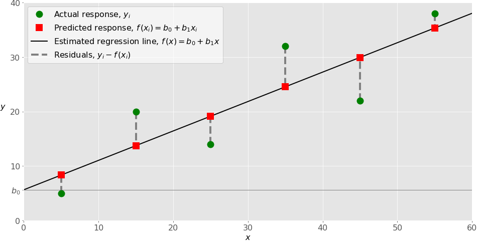
If our model's assumptions are met and it's a good fit for the data, the residuals should be randomly scattered around zero with no obvious patterns. Let's explore the two most important diagnostic plots.
The following article from The Programming Historian provides an exceptionally clear guide to validating a linear regression model by analyzing its residuals.
Regression Analysis with Scikit-Learn (part 1 - Linear)
This article offers a detailed, step-by-step guide to model validation through visual inspection.
Read the section titled Step 9: Model Validation. Focus your attention on these two parts: Distribution of Residuals: Read the explanation and study the code for creating a DataFrame of results and plotting a histogram/KDE plot of the residuals. A well-behaved model will have residuals that are roughly normally distributed around zero. Homoscedasticity: Read this subsection to understand why we want the error variance to be constant. Study the code and the interpretation of the scatter plot of predicted vs. actual values. This plot is perhaps the single most useful diagnostic for a regression model.
By creating and interpreting these plots, you move beyond simply looking at a single R² score. You start to diagnose how your model is failing.
- Does the residual plot show a U-shape? This might indicate that the true relationship is non-linear, and a simple linear model is insufficient (high bias).
- Does the actual vs. predicted plot show that errors get larger as the predicted value increases (a funnel shape)? This is called heteroscedasticity and violates a key assumption of linear regression.
These visual checks, combined with your quantitative metrics, provide a comprehensive picture of your model's performance.
Conclusion
In this lesson, you've bridged the gap between theory and practice. You took the concepts of linear regression and evaluation and applied them in a concrete, end-to-end workflow using scikit-learn.
Key Takeaways:
- The standard workflow for applying a supervised model involves loading data, splitting it into training and testing sets, fitting the model on the training data, and making predictions on the test data.
- Model evaluation is a multi-faceted process that requires both quantitative metrics (like MSE, RMSE, and R²) and visual diagnostics.
- The Actual vs. Predicted plot is a powerful tool to quickly assess model fit. Ideally, the points should form a tight, straight line along the
y=xaxis. - The Residual Plot helps you check the assumptions of linear regression. For a good model, residuals should appear as a random cloud of points with no discernible patterns.
In the videos and articles, you saw that once a model is trained, we can access its coef_ and intercept_ attributes. In our next lesson, we will focus entirely on interpreting these coefficients. You will learn how to use them to understand the relationships between the features and the target, moving from just predicting a value to explaining what drives that value.