Hello! In our last session, we mastered cross-validation, a robust technique for getting a reliable estimate of a model's performance on unseen data. We saw that a single train-test split can be misleading, and that by averaging scores across multiple "folds," we gain a much more trustworthy picture of our model's generalization error.
Today, we'll dissect that error. We'll explore one of the most fundamental concepts in all of machine learning: the bias-variance tradeoff. You will learn how the total error of any model can be broken down into three components: bias, variance, and an irreducible error. Understanding this decomposition is the key to diagnosing the two most common failure modes of machine learning models: underfitting and overfitting. This lesson provides the theoretical framework you'll use throughout this course to understand why a model works, why it fails, and how to improve it.
The Problem of Model Complexity
At the heart of machine learning is a central tension. We want a model that is flexible enough to capture the true, underlying patterns in our data. However, we also want a model that is not so flexible that it starts learning the random noise inherent in the data, which would cause it to perform poorly on new, unseen examples.
This leads to two opposing problems:
- Underfitting: The model is too simple and fails to capture the underlying structure of the data. It performs poorly on both the data it was trained on and new data.
- Overfitting: The model is too complex and learns the training data too well, including its random noise. It performs exceptionally well on the training data but fails to generalize to new data.
Let's start with a classic, intuitive explanation of this dilemma from StatQuest.
Machine Learning Fundamentals: Bias and Variance
This video, "Machine Learning Fundamentals: Bias and Variance," uses a simple and effective analogy of fitting a line to data about mice to explain underfitting and overfitting.
Watch from the beginning until the introduction of overfitting. Pay close attention to the two types of models presented: The straight line: Notice how its inflexibility prevents it from capturing the true curved relationship. This is a model with high bias. The squiggly line: Observe how its extreme flexibility allows it to fit the training data perfectly but results in a terrible fit for the test data. This is a model with high variance.
The video brilliantly illustrates the core issue. The simple linear model is biased; its assumption of a linear relationship is fundamentally wrong for this data. The complex "squiggly" model has high variance; its predictions would change wildly if we gave it a slightly different set of training points. The ideal model is somewhere in between.
A Visual Metaphor: The Target Analogy
To solidify the concepts of bias and variance, let's use a popular analogy: a target. Imagine the bullseye is the true value we want our model to predict. Each time we train our model on a different subset of data, we get a slightly different model, which produces a new prediction (a shot at the target).

Let's break down the four scenarios shown in the image:
- Low Bias, Low Variance (Top-Left): This is the ideal scenario. The predictions are accurate (centered around the bullseye) and consistent (tightly clustered). This is what we strive for in a good model.
- High Bias, Low Variance (Bottom-Left): The model is consistent but inaccurate. Its predictions are tightly clustered but systematically miss the bullseye. This corresponds to an underfit model, like the straight line from the video. It makes strong, simple assumptions that are incorrect, leading to a consistent error.
- Low Bias, High Variance (Top-Right): The model is "correct" on average (the shots are centered around the bullseye) but is very inconsistent. Each prediction is far from the others. This corresponds to an overfit model, like the squiggly line. It is highly sensitive to the specific training data it saw, causing its predictions to be scattered.
- High Bias, High Variance (Bottom-Right): This is the worst-case scenario. The model is both inaccurate and inconsistent.
Decomposing the Error: The Mathematical View
This tradeoff isn't just a conceptual idea; it has a firm mathematical foundation. For many common loss functions, like Mean Squared Error (MSE), the expected error of a model on unseen data can be decomposed as follows:
Let's define these terms more formally:
- Bias²: The squared difference between the average prediction of our model (if we were to train it on many different training sets) and the true value we are trying to predict. It measures how much the model's average prediction deviates from the correct value.
- Variance: The variability of a model's prediction for a given data point. It measures how much the predictions would change if we used a different training set.
- Irreducible Error: This component is due to the inherent noise or randomness in the data itself. No matter how good our model is, we can never get rid of this error. It represents a lower bound on the error for any model.
The following interactive article provides a fantastic, step-by-step visualization of this decomposition.
Bias Variance Tradeoff - MLU-Explain
This MLU-Explain article visualizes the entire process, from underfitting and overfitting to the final tradeoff curve.
Work your way through the article sequentially. Focus on these key sections: Read the section on underfitting. Notice how the simple model has high error on both training and test data. Continue to the section on overfitting. See how the complex model achieves zero training error but has a very high test error. Next, study the sections on Bias and Variance. These provide the formal definitions and connect them back to the underfit and overfit models. Finally, read through the rest of the explanation, which aggregates these concepts into the final U-shaped curve, beautifully illustrating the tradeoff.
The key insight is that as you increase model complexity (e.g., using a higher-degree polynomial in regression, or a more flexible "squiggly line"), you are trading bias for variance.
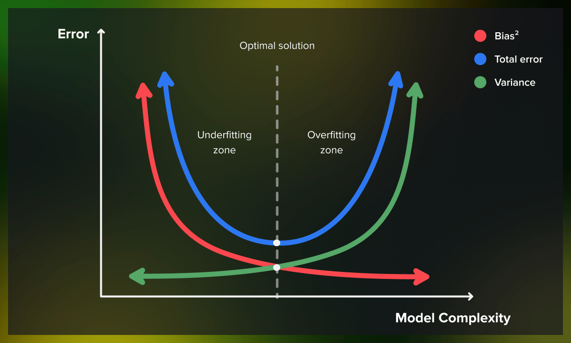
As the graph shows:
- Simple models (left side): Have high bias and low variance. They are underfitting.
- Complex models (right side): Have low bias and high variance. They are overfitting.
- The sweet spot (middle): The optimal model has a balanced combination of bias and variance that minimizes the total error.
Diagnosing High Bias vs. High Variance
So, how do you know if your model is suffering from high bias or high variance in practice? You can diagnose it by comparing the model's performance on the training set versus the validation/test set. The cross-validation skills you learned in the last lesson are your primary tool here.
- High Bias (Underfitting): The model performs poorly on both the training set and the test set. A high training error is the tell-tale sign. The model is too simple to even learn the patterns in the data it was trained on.
- High Variance (Overfitting): The model performs very well on the training set but poorly on the test set. A large gap between a low training error and a high test error is the classic symptom. The model has memorized the training data instead of learning generalizable patterns.
This brief article from IBM reinforces these diagnostic symptoms.
What is Bias-Variance Tradeoff?
This article provides another clear overview of the topic. We'll focus on the section that summarizes the symptoms of high-bias and high-variance models.
Read the section titled Bias and variance in practice. This provides a concise summary of the symptoms and common examples of high-bias (underfitting) and high-variance (overfitting) models.
Conclusion
You've just explored one of the most critical balancing acts in machine learning. Without a firm grasp of the bias-variance tradeoff, it's easy to misinterpret a model's performance and make poor modeling decisions.
Key Takeaways:
- Model error on unseen data is composed of Bias, Variance, and Irreducible Error.
- Bias is a systematic error caused by a model's simplifying assumptions. High bias leads to underfitting.
- Variance is an error caused by a model's sensitivity to the specific training data. High variance leads to overfitting.
- There is a tradeoff: increasing model complexity typically decreases bias but increases variance.
- The goal is not to eliminate bias or variance entirely, but to find a balance that minimizes the total error.
- You can diagnose these issues by comparing training error and test error:
- High training error & high test error → High Bias
- Low training error & high test error → High Variance
In our next lesson, we will finally apply linear regression to a real-world dataset. You'll not only build and evaluate the model but also start to interpret its results. Your understanding of cross-validation and the bias-variance tradeoff will be your guiding framework for assessing its performance and considering potential improvements.