Ridge and Lasso Regression: Regularization in Practice

The Practical Workflow: From Data to Interpretation

Before diving into the code, let's outline the key steps we will follow. This workflow is standard for applying regularized models:

1. Load and Prepare Data: We'll import a dataset and perform some initial exploration.
2. Split and Scale: We'll split the data into training and testing sets. Crucially, we will then scale our features. This is a vital step for regularization, as the penalties are applied directly to the coefficients. If features are on vastly different scales (e.g., one from 0-1 and another from 10,000-50,000), the penalty would unfairly punish the coefficients of the larger-scaled features. Standardization ensures all features are treated equally by the regularization term.
3. Train a Baseline Model: We'll fit a standard LinearRegression model to serve as our baseline for comparison.
4. Train Regularized Models: We'll fit Ridge and Lasso models to the same data.
5. Compare and Interpret: The final and most important step is to compare the coefficients and performance scores of all three models to understand the distinct effects of L1 and L2 regularization.

We will use a comprehensive tutorial from DataCamp as our guide for this practical exercise. It provides all the necessary code and context using the Boston housing dataset, a classic dataset for regression tasks.

Applying Ridge Regression and Observing Shrinkage

With our data prepared, our first step is to train a standard linear regression model and a Ridge regression model. This will allow us to directly compare their coefficients and see the "shrinking" effect of the L2 penalty in action.

The comparison plot you just examined is the key to interpretation. The unregularized linear regression model may have large coefficient values, suggesting it's placing a great deal of importance on certain features. This can be a sign of overfitting, where the model is too closely tuned to the noise in the training data. Ridge regression mitigates this by "pulling" all coefficients towards zero, resulting in a less complex model that often generalizes better to unseen data.

Applying Lasso Regression and Witnessing Feature Selection

Now, let's turn our attention to Lasso (L1) regression. While it also shrinks coefficients, its main distinguishing feature is its ability to shrink some of them to exactly zero. This effectively removes the corresponding features from the model, performing automatic feature selection.

Let's see what happens when we apply Lasso with a strong penalty.

This result perfectly illustrates the double-edged nature of the alpha hyperparameter. A value that is too high can lead to an over-penalized, underfitting model. This begs the question: how do we find the optimal value for alpha?

Visualizing the Regularization Path

Before we answer that question, it's helpful to visualize what happens to the coefficients as we vary the regularization strength. A "regularization path" plot shows the magnitude of each feature's coefficient as a function of alpha.

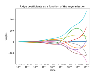
This visualization makes the trade-off clear. A very high alpha (right side of the plot) results in a simple model with small coefficients. As alpha decreases, the model becomes more complex, allowing the coefficients to take on larger values that better fit the training data. Our goal is to find the "sweet spot" that balances this complexity to achieve the best performance on unseen data.

Finding the Optimal Alpha with Cross-Validation

Manually testing different values for alpha is tedious and unreliable. The standard, robust method for tuning this hyperparameter is to use cross-validation. Scikit-learn provides convenient classes, LassoCV and RidgeCV, that automatically perform this process for us. These models test a range of alpha values using cross-validation and select the one that performs best.

Let's see this in action with LassoCV.

This final plot is the culmination of our work. By comparing the three sets of coefficients, you can concretely interpret the impact of each regularization strategy on the model.

To connect this practical result back to the theory, let's briefly revisit the geometric interpretation.

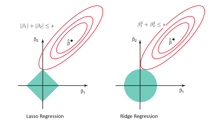
The coefficient plots you just generated are a direct consequence of this geometry.

• Ridge's circular constraint means that the loss function's ellipse will almost always touch the boundary at a point where no coefficient is zero. This leads to shrinkage without feature elimination.
• Lasso's diamond-shaped constraint has sharp corners that lie on the axes. The ellipse often makes its first contact at one of these corners, forcing the coefficient for the other axis to become exactly zero. This is the geometric basis for Lasso's feature selection property.

For a final reinforcement of this geometric intuition, you can review the following short explanation.

Conclusion

In this lesson, you successfully bridged the gap between the theory of regularization and its practical application. You used scikit-learn to apply Ridge and Lasso regression to a dataset, seeing firsthand how they modify model coefficients to combat overfitting.

Key Takeaways:

• Feature scaling is a mandatory preprocessing step before applying regularized models.
• Ridge (L2) regression shrinks the coefficients of all features, reducing model complexity and helping with multicollinearity. All features remain in the model.
• Lasso (L1) regression also shrinks coefficients but has the unique ability to force some to exactly zero, performing automatic feature selection.
• The alpha hyperparameter controls the strength of the penalty. A value that is too large can cause underfitting.
• RidgeCV and LassoCV are the standard tools for efficiently finding the optimal alpha value using cross-validation.
• By plotting and comparing coefficients, you can directly interpret the impact of regularization and gain insights into which features are being prioritized or eliminated.

In our next lesson, we will complete our practical exploration by applying Elastic Net regression. We will then compare its performance against Ridge, Lasso, and standard linear regression, solidifying your ability to choose and apply the best model for a given scenario.