Welcome to the next step in our exploration of unsupervised learning. In the last lesson, we tackled the crucial question of how to choose the optimal number of clusters, K, for the K-Means algorithm. We learned about the elbow method, which looks for a point of diminishing returns in WCSS, and the more robust silhouette score, which measures cluster cohesion and separation.
Today, we will put that theory into practice. Your goal for this course includes not just understanding the algorithms but applying them to real datasets, and this lesson is designed to do exactly that. We will walk through a complete, end-to-end K-Means clustering project. This involves loading and preparing a dataset, using the elbow method to determine an appropriate K, fitting the K-Means model, and, most importantly, visualizing the results to interpret the patterns the algorithm has discovered.
The Clustering Pipeline: A Practical Walkthrough
Our goal is to segment customers from a mall based on their annual income and spending habits. This is a classic marketing analytics task where clustering helps identify distinct customer groups for targeted strategies. We will use a popular dataset, often called the "Mall Customer" dataset, for this purpose.
The article "How to Perform KMeans Clustering Using Python" on Towards Data Science provides a straightforward guide for this task, which we will use as the backbone for our practical exercise.
1. Loading and Preparing the Data
First, we need to load the data and select the features we'll use for clustering. For this problem, we are most interested in the numerical features that describe customer behavior: Annual Income and Spending Score.
How to Perform KMeans Clustering Using Python
This article will guide our implementation. We'll start with loading and selecting the data. The dataset customer_data.csv used in the article is a standard one you can find on platforms like Kaggle under the name "Mall Customer Segmentation Data". For this lesson, you can assume you have it downloaded.
Begin by reading the sections that cover loading the data and selecting the relevant columns. This sets up our initial DataFrame in pandas.
2. The Importance of Feature Scaling
As you'll recall, the K-Means algorithm is fundamentally based on calculating distances between data points and centroids. If our features are on vastly different scales (e.g., income in tens of thousands and a spending score from 1-100), the feature with the larger scale will dominate the distance calculation, unduly influencing the clustering.
To prevent this, we must scale our features. Standardization (or Z-score scaling), which you've used in supervised learning, is a perfect tool for this. It rescales each feature to have a mean of 0 and a standard deviation of 1, ensuring all features contribute equally to the distance metric.
The video below gives an excellent justification for why scaling is so critical in the context of K-Means.
Hands On Data Science Project: Understand Customers with KMeans Clustering in Python
This video project from TrentDoesMath clearly explains the necessity of scaling before applying K-Means.
Watch the segment from this video where the presenter discusses the sensitivity of K-Means to feature scales and introduces standard scaling as the solution. Following this, watch the implementation part from the video to see how to apply the StandardScaler from scikit-learn to a pandas DataFrame.
Now, let's apply this step to our own data, following the guidance from our main article.
How to Perform KMeans Clustering Using Python
This section covers the practical application of StandardScaler.
Read the section on data transformation. Implement this code to scale the Annual Income and Spending Score columns.
3. Determining the Optimal K
With our data scaled, we can now apply the techniques from our previous lesson. We'll generate an elbow plot to find a suitable value for K. The plot will show the algorithm's inertia (WCSS) for a range of K values. We're looking for the "elbow"—the point where the inertia stops decreasing sharply.

Let's generate this plot for our customer dataset.
How to Perform KMeans Clustering Using Python
This part of the article provides the code to implement the elbow method.
Follow the instructions in the section "Determine the best number of cluster". This involves creating a loop to run K-Means for different values of k, storing the inertia_ for each, and then plotting the results. Based on the resulting plot for the mall customer data, K=5 appears to be the optimal choice.
4. Applying K-Means and Visualizing the Clusters
We've done the prep work: our data is scaled and we have our optimal number of clusters, K=5. Now it's time to run the K-Means algorithm one final time and visualize the customer segments it identifies.
The process is as follows:
- Initialize the
KMeansmodel fromsklearn.clusterwithn_clusters=5. - Fit the model to your scaled data.
- The cluster assignments for each data point will be stored in the
.labels_attribute of the fitted model. - Create a scatter plot of the original (unscaled)
Annual Incomevs.Spending Score. - Color each point on the scatter plot according to its assigned cluster label.
This final visualization is the payoff—it allows us to visually inspect and interpret the customer segments.
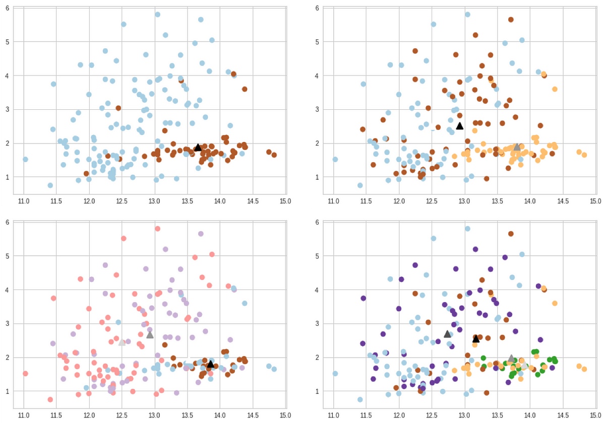
Now, let's perform the final fit and visualization.
How to Perform KMeans Clustering Using Python
The final sections of the article show how to fit the model and visualize the results.
First, read and implement the code in the section "Create the final KMeans model". This will fit the model with K=5 and add the resulting labels to your DataFrame. Next, use the code in the final section, "Visualize the clusters", to generate the scatter plot. This plot is the direct output of your work and the key deliverable of this lesson.
The resulting scatter plot should clearly show five distinct groups of customers. For example, you might see a high-income, low-spending group; a low-income, high-spending group; and a group that is average on both metrics. These are actionable insights that a business could use for marketing campaigns.
For an even more rigorous analysis, you could create violin plots for each feature, broken down by cluster. This helps you precisely characterize the distribution of features within each segment and give them meaningful names like "High-Value Spenders" or "At-Risk Savers". The video from TrentDoesMath provides a fantastic example of this advanced interpretation step.
Hands On Data Science Project: Understand Customers with KMeans Clustering in Python
This part of the video demonstrates how to use violin plots for a deep-dive analysis of the clusters.
Watch the final segment from this video. The presenter analyzes the distribution of each feature within each cluster and uses these insights to assign meaningful, business-relevant names to the segments. This is an excellent example of moving from a technical result to a strategic insight.
Conclusion
Congratulations! You have successfully executed a complete K-Means clustering pipeline. You started with a raw dataset, made a critical preprocessing decision by scaling your features, used a data-driven method to select the optimal number of clusters, and generated and visualized the final customer segments. This workflow is a foundational skill in unsupervised machine learning.
Key Takeaways:
- End-to-End Workflow: Applying K-Means involves a standard sequence: data loading, feature selection, preprocessing (especially scaling), determining K, fitting the model, and visualization/interpretation.
- Feature Scaling is Non-Negotiable: Because K-Means is distance-based, you must scale your features to prevent features with larger magnitudes from dominating the algorithm.
- Visualization is Key: Clustering results are often best understood visually. A simple scatter plot, colored by cluster, can reveal powerful insights about the underlying structure of your data.
- Interpretation is the Goal: The final step is to interpret what the clusters mean in the context of the problem. What defines each group? What are their characteristics? This transforms the output of an algorithm into actionable business intelligence.
What's Next:
K-Means is an excellent and widely used clustering algorithm, but it has its limitations. It tends to find spherical clusters and struggles with complex shapes or clusters of varying densities. Furthermore, the need to specify K beforehand can sometimes be a disadvantage.
In our next lesson, we will explore Hierarchical Agglomerative Clustering. This method takes a different approach, building a hierarchy of clusters from the bottom up. It doesn't require you to pre-specify K and allows you to visualize the entire cluster hierarchy using a powerful tool called a dendrogram.