Hello! In our previous lesson, we dove into the mechanics of the K-Means algorithm, exploring its iterative process of assigning data points and updating centroids to form clusters. We concluded with a critical unanswered question: how do we determine the right number of clusters, K, to begin with?
This lesson directly addresses that challenge. Your choice of K fundamentally determines the structure K-Means will find in your data. Choosing a value that is too low can merge distinct groups, while choosing one that is too high can artificially split natural clusters. Today, we will explore two of the most common and effective techniques for selecting an optimal value for K: the elbow method and the silhouette score. Mastering these methods is a key step in moving from understanding how an algorithm works to applying it effectively in practice.
The Elbow Method: Finding the Point of Diminishing Returns
The first technique, the elbow method, is a visual heuristic based on a simple trade-off. As we increase the number of clusters (K), the data points within each cluster will naturally get closer to their respective centroids. We can measure this "tightness" or "compactness" using a metric called the Within-Cluster Sum of Squares (WCSS). In scikit-learn, this is also referred to as inertia.
WCSS is calculated as the sum of the squared distances between each data point and the centroid of its assigned cluster.
where is the i-th cluster, is a data point in that cluster, and is the centroid of cluster .
The core idea of the elbow method is to run K-Means for a range of K values (e.g., from 1 to 10) and plot the WCSS for each. As K increases, WCSS will always decrease. However, at some point, adding more clusters provides diminishing returns—the drop in WCSS becomes much less significant. We look for this point on the graph, which often resembles an "elbow".
K-Means Clustering in Python: A Practical Guide
This article from Real Python provides a concise explanation and implementation of both the elbow method and the silhouette coefficient.
First, focus on the section "Choosing the Appropriate Number of Clusters". Read the part that introduces the elbow method, starting from the initial explanation. Then, examine the code block that calculates the SSE (Sum of Squared Errors, another name for WCSS) for different values of k. Pay attention to how kmeans.inertia_ is used to get the WCSS value. Finally, look at the interpretation of the plot and the resulting graph, which clearly shows an "elbow".
While intuitive, the elbow method has a significant drawback: the "elbow" is often ambiguous and hard to identify, especially in complex, high-dimensional datasets. It becomes a subjective judgment call.
The article "Elbow Method: Definition, Drawbacks, vs. Silhouette Score" discusses this limitation clearly.
Elbow Method: Definition, Drawbacks, vs. Silhouette Score | Built In
This article from Built In provides a great conceptual breakdown of the elbow method and its common pitfalls.
Read the section "What Is the Elbow Method?" for a recap of the concept. Then, pay close attention to the next section, "What Are the Drawbacks?", which illustrates the difference between an ideal elbow curve and what you often see in practice.
The Silhouette Score: Measuring Cohesion and Separation
To address the ambiguity of the elbow method, we can turn to a more robust metric: the silhouette score. This score evaluates the quality of clustering by measuring how well each data point fits into its assigned cluster compared to other clusters. It considers two crucial factors:
- Cohesion (): The average distance from one data point to all other points in the same cluster. A small value of means the cluster is dense and well-grouped.
- Separation (): The average distance from that same data point to all points in the nearest neighboring cluster. A large value of means the cluster is well-separated from other clusters.
For a single data point , the silhouette score is calculated as:
The score ranges from -1 to +1:
- +1: Indicates the data point is perfectly clustered—far from neighboring clusters and very close to points in its own cluster.
- 0: Indicates the data point is on or very close to the boundary between two clusters.
- -1: Indicates the data point may be assigned to the wrong cluster, as it is closer to a neighboring cluster than its own.
To evaluate the entire clustering for a given K, we compute the average silhouette score across all data points. Unlike the elbow method, where we look for a "kink," here we simply look for the value of K that maximizes the average silhouette score.
The following video provides an excellent intuitive breakdown of this calculation.
Live Day 6- Discussing KMeans,Hierarchical And DBScan Clustering Algorithms
In this segment, Krish Naik explains the intuition behind the silhouette score as a validation metric for clustering.
Watch the portion from this video where he discusses how to validate clustering models. He provides a clear, step-by-step explanation of: The calculation of a(i) (intra-cluster distance). The calculation of b(i) (inter-cluster distance). The final silhouette score formula and its interpretation based on the relationship between a(i) and b(i).
Visualizing Silhouette Scores
Beyond just an average score, we can create silhouette plots to get a deeper diagnostic view. A silhouette plot displays the silhouette score for every single sample in the dataset, sorted and grouped by cluster.

When analyzing a silhouette plot, you should look for two things:
- Positive Scores: All clusters should have scores above the average silhouette score (the red line). Any samples dipping into negative values are likely misclassified.
- Uniform Thickness: The "blades" of the plot for each cluster should have similar thickness, indicating that the clusters are of a relatively uniform size. Wide fluctuations can suggest that a large cluster has been artificially split or that several smaller groups have been merged.
The article from Real Python we looked at earlier also has a great section on implementing this.
K-Means Clustering in Python: A Practical Guide
This part of the article demonstrates how to calculate and interpret the average silhouette score.
Return to the "Choosing the Appropriate Number of Clusters" section and read the part on the silhouette coefficient. Observe the code that calculates the score for different values of k and how the plot is used to identify the optimal k (the one with the highest score).
Combining Methods for a Robust Decision
In practice, it's rarely a good idea to rely on a single metric. A common and effective workflow is to use both the elbow method and the silhouette score to guide your choice of K. You can plot both metrics on the same graph to get a consolidated view.
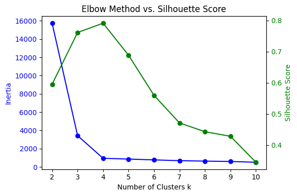
When interpreting a plot like this, you look for a value of K that represents a good compromise:
- It should be at or near the "elbow" of the inertia curve (blue line).
- It should correspond to a high (ideally the peak) silhouette score (green line).
In the plot above, K=4 appears to be a strong candidate. The inertia curve has a distinct elbow at K=4, and the silhouette score is at its absolute peak. While K=3 also shows a sharp drop in inertia, the silhouette score is significantly lower, suggesting the clusters at K=4 are better separated.
The video below provides a full practical walkthrough, implementing both methods in Python to arrive at a final choice for K.
k-means Elbow Method and Silhouette Method
This video by Kunaal Naik demonstrates the end-to-end process of using both the elbow and silhouette methods to find the optimal number of clusters.
First, watch the implementation of the elbow method. Notice how the WCSS (inertia_) is calculated for a range of K and then plotted. Next, see how the silhouette method is implemented. The goal here is to find the value of K that maximizes the score. Finally, watch how the results are validated. The video confirms that both methods point to the same optimal K, giving confidence in the result.
Conclusion
You now have a robust toolkit for one of the most critical steps in K-Means clustering: selecting the optimal number of clusters. While there's no single "magic" answer, using these data-driven techniques moves you from guesswork to an informed, justifiable decision.
Key Takeaways:
- The Problem with K: The number of clusters, K, is a hyperparameter that must be chosen by the user, and it heavily influences the outcome of the K-Means algorithm.
- Elbow Method: A heuristic that plots WCSS (inertia) against different values of K. The optimal K is at the "elbow," the point of diminishing returns where adding more clusters doesn't significantly reduce WCSS. Its main weakness is ambiguity.
- Silhouette Score: A more robust metric that quantifies how well-suited each point is to its cluster by measuring both cohesion (intra-cluster similarity) and separation (inter-cluster dissimilarity). The optimal K is the one that maximizes the average silhouette score.
- Practical Approach: Use both methods together. Look for a K value that corresponds to an elbow in the WCSS plot and a peak in the silhouette score plot.
What's Next:
With the theory of K-Means and the methods for selecting K now covered, it's time to put it all into practice. In the next lesson, you will apply K-Means clustering to a real-world dataset, use the elbow and silhouette methods to determine the optimal number of clusters, and visualize the final result.