Hierarchical Clustering and Dendrogram Interpretation

From Points to a Hierarchy

At its core, hierarchical clustering creates a tree-like structure of clusters, known as a dendrogram. There are two main approaches to this:

1. Agglomerative (Bottom-Up): This is the most common approach and the focus of our lesson. It starts by treating every single data point as its own cluster. Then, it iteratively merges the two "closest" clusters until only one large cluster, containing all data points, remains.
2. Divisive (Top-Down): This method works in the opposite direction. It starts with all data points in a single cluster and recursively splits them into smaller clusters until each point is in its own cluster. This method is more computationally complex and less frequently used in practice.

The following video from 365 Data Science provides a concise overview of these two approaches and sets the stage for our deep dive into the agglomerative method.

The Agglomerative Clustering Algorithm

Given your background in algorithms, you can think of the agglomerative process as a greedy algorithm that builds a binary tree. At each step, it makes the locally optimal choice of merging the two most similar clusters. Let's break down the process.

A superb and very clear explanation of this iterative process is provided in the StatQuest video below.

To formalize the intuition from the video, the algorithm proceeds as follows:

1. Initialization: Begin by assigning each data point to its own cluster. If you have N data points, you start with N clusters.
2. Compute Proximity: Calculate a distance matrix containing the distance between every pair of clusters. Initially, this is just the distance between each pair of individual points (e.g., using Euclidean distance).
3. Merge: Find the two closest clusters in the distance matrix and merge them into a single new cluster.
4. Update: Update the distance matrix. Remove the entries for the two old clusters and add new entries for the newly formed cluster. The distances between this new cluster and the others are calculated using a linkage criterion.
5. Repeat: Repeat steps 3 and 4 until only one cluster remains.

The article "Hierarchical Clustering: Complete Guide with Dendrograms" provides a rigorous breakdown of these steps.

Defining "Closeness": Distance and Linkage

The algorithm repeatedly merges the "closest" clusters. But how do we define the distance between two clusters, which might contain many points? This is determined by two key choices: the distance metric and the linkage criterion.

• Distance Metric: This measures the distance between two individual data points. The most common is Euclidean distance, which you've encountered before. Others include Manhattan distance. Your choice of metric defines the space in which similarity is measured.

• Linkage Criterion: This defines how to measure the distance between two clusters. This is a crucial hyperparameter in hierarchical clustering. The choice of linkage criterion dictates which clusters are merged and, consequently, the shape of the final clusters.

Here are the five most common linkage criteria:

1. Single Linkage: The distance between two clusters is the minimum distance between any two points in the two clusters. It's good at handling non-elliptical shapes but can be sensitive to noise and outliers, sometimes creating long, stringy clusters (a phenomenon known as the "chaining effect").
2. Complete Linkage: The distance between two clusters is the maximum distance between any two points in the two clusters. It tends to produce more compact, spherical clusters and is less susceptible to noise.
3. Average Linkage: The distance is the average of the distances between all pairs of points from the two clusters. It provides a balance between the sensitivity of single linkage and the compactness of complete linkage.
4. Centroid Method: The distance is measured between the centroids (mean vectors) of the two clusters.
5. Ward's Method: This is a popular and effective choice. It merges the two clusters that result in the smallest increase in the total within-cluster variance. Essentially, it tries to find the most compact, spherical clusters.

The StatQuest video explains the concept of distance metrics and linkage criteria very clearly.

The Dendrogram: Reading the Cluster Tree

The entire merging process of hierarchical clustering is captured in a single, powerful visualization: the dendrogram.

The dendrogram shows the sequence of merges and the distance at which each merge occurred.

• The leaves (at the bottom) are the individual data points.
• As you move up, horizontal lines connect clusters (or points) that have been merged.
• The height of the horizontal line on the y-axis represents the distance (or dissimilarity) between the two clusters when they were merged. A taller line signifies that two more dissimilar clusters were merged.

The 365 Data Science video provides an excellent walkthrough of reading a dendrogram using a real-world example.

From Dendrogram to Clusters

A key advantage of hierarchical clustering is that you don't need to specify the number of clusters beforehand. Instead, you decide the number of clusters after the algorithm has run by analyzing the dendrogram.

The method is to "cut" the dendrogram at a certain height. The number of vertical lines your horizontal cut intersects determines the number of clusters.

So, where should you cut? The most common heuristic is to find the longest vertical line that is not crossed by any horizontal lines. You then draw your horizontal cut through this gap. The intuition is that a long vertical line represents a large distance jump, indicating that you just merged two very different clusters. This suggests that the clusters before that merge were distinct and well-separated.

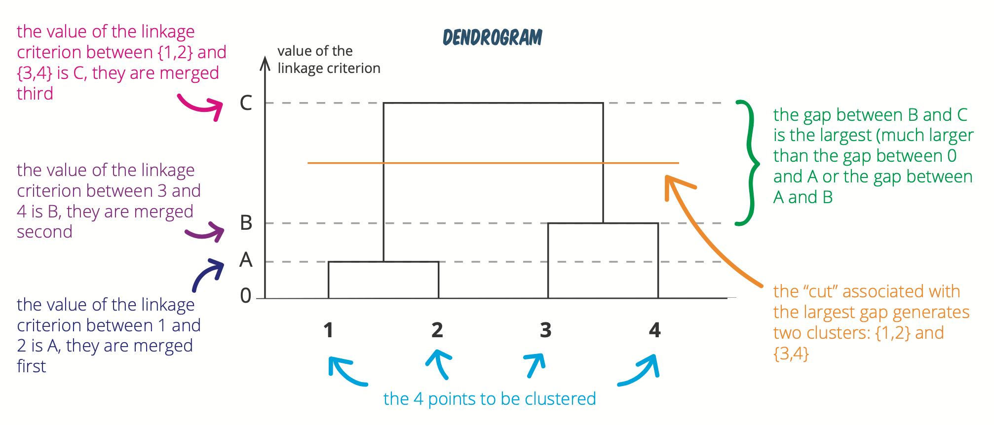
The article "Hierarchical Clustering: Agglomerative and Divisive Explained" has a very clear demonstration of this cutting technique.

To see this logic in action, let's look at one final, simple example that ties everything together.

Conclusion

In this lesson, we have unpacked the theory behind Hierarchical Agglomerative Clustering. Unlike K-Means, which partitions data based on a fixed K, HAC builds a complete hierarchy of clusters, offering a more nuanced view of the relationships within your data.

Key Takeaways:

• Hierarchical Agglomerative Clustering (HAC) is a "bottom-up" algorithm that starts with individual points and iteratively merges the closest clusters.
• The process does not require you to pre-specify the number of clusters.
• The "closeness" of clusters is defined by a distance metric (e.g., Euclidean) and a linkage criterion (e.g., Ward, complete, average).
• The entire merge history is visualized in a dendrogram, a tree-like diagram where the height of branches indicates the dissimilarity between merged clusters.
• To determine the optimal number of clusters, you "cut" the dendrogram horizontally at the level of the largest vertical gap. The number of vertical lines intersected by the cut is your number of clusters.

What's Next:

Now that you understand the theory, the next logical step is to apply it. In the next lesson, we will implement hierarchical clustering in Python. You'll take a dataset, generate a dendrogram to decide on the optimal number of clusters, and then apply the AgglomerativeClustering model from scikit-learn to segment the data.