Kernel Trick: SVMs for Non-Linear Data

The Problem: When a Straight Line Isn't Enough

Linear SVMs are powerful, but they are limited to finding a linear decision boundary. What happens when your data looks like this?

As you can see, no straight line in the 2D plane can separate the red squares from the green circles. A linear model would fail. The intuitive solution, as shown in the image, is to project the data into a higher dimension. In this new, higher-dimensional space, the data might become linearly separable. A separating hyperplane in this new space, when projected back down to the original, lower-dimensional space, corresponds to a complex, non-linear decision boundary.

This concept of adding dimensions to make data separable is explained very clearly in the following video from StatQuest. It uses a simple 1D example that is impossible to separate but becomes trivial in 2D.

The "Trick": Efficiency is Key

The idea of adding features to create a higher-dimensional space is not unique to SVMs. You could, for example, manually create new polynomial features (like $x_1^2$, $x_2^2$, $x_1{x}_2$, etc.) and then feed them into a linear model. However, this has two major drawbacks:

1. Computational Cost: If you map your data to a very high-dimensional space, the number of computations can become enormous.
2. Feature Selection: How do you know which transformation to apply? Should you use squared terms, cubic terms, or something else entirely?

This is where the genius of the kernel trick comes in. If you recall the SVM optimization problem from our last lesson, you'll remember that the algorithm's calculations (both for finding the hyperplane and for classifying new points) depend only on the dot product between pairs of data points (${\mathbf{x}}_i\cdot {\mathbf{x}}_j$).

The kernel trick is based on a simple but powerful observation: we don't need to know the coordinates of our data in the high-dimensional space; we only need to know the dot products between them in that space.

A kernel is a function $K$ that takes two vectors in the original space, ${\mathbf{x}}_i$ and ${\mathbf{x}}_j$, and returns the dot product of their images in the high-dimensional space, $\varphi ({\mathbf{x}}_i)\cdot \varphi ({\mathbf{x}}_j)$.

The "trick" is that we can compute this kernel function $K({\mathbf{x}}_i,{\mathbf{x}}_j)$ efficiently in the original, low-dimensional space, completely bypassing the expensive step of explicitly transforming the data.

The following short video explains this crucial concept succinctly.

Common Kernel Functions

Now that you understand what the kernel trick does, let's look at the two most common kernels you'll encounter. For this, we'll turn to a resource that lays out their mathematical form, which aligns with your goal of getting a "working understanding" of the math.

Let's dissect what you just read:

1. Polynomial Kernel

The polynomial kernel is defined as:
$K({\mathbf{x}}_i,{\mathbf{x}}_j)=(\gamma {\mathbf{x}}_i^T{\mathbf{x}}_j+r{)}^d$
This kernel essentially computes the dot product in a feature space composed of polynomials of degree up to $d$.

• d (degree): This is the key hyperparameter. It controls the flexibility of the decision boundary. A degree of 1 makes it a linear kernel. A higher degree like 2 or 3 allows for more complex, curved boundaries by implicitly creating interaction features (e.g., $x_1{x}_2$) and polynomial features (e.g., $x_1^2$).
• r (coef0): This is a coefficient that trades off the influence of higher-order versus lower-order terms in the polynomial.
• γ (gamma): A scaling coefficient for the dot product.

2. Radial Basis Function (RBF) Kernel

The RBF kernel is the most popular choice for SVMs and is defined as:
$K({\mathbf{x}}_i,{\mathbf{x}}_j)=\exp (-\gamma ||{\mathbf{x}}_i-{\mathbf{x}}_j|{|}^2)$
As the video mentioned, the RBF kernel maps data to an infinite-dimensional space. This would be impossible without the kernel trick.

• Intuition: The RBF kernel can be thought of as a similarity measure. Its value is close to 1 if two points ${\mathbf{x}}_i$ and ${\mathbf{x}}_j$ are very close (i.e., the distance $||{\mathbf{x}}_i-{\mathbf{x}}_j|{|}^2$ is small), and it decays towards 0 as the points get farther apart.
• γ (gamma): This hyperparameter defines how much influence a single training example has.
  • A low gamma means a large similarity radius, so points farther apart are considered similar. This results in a smoother, more general decision boundary.
  • A high gamma means a small similarity radius. Only points very close to each other are considered similar. This can lead to a more complex, "wiggly" boundary that might overfit the training data.

Kernels in Action

The best way to understand the effect of different kernels is to see them in action. The following image shows four different kernels (Linear, RBF, Polynomial, Sigmoid) applied to three different non-linear datasets.

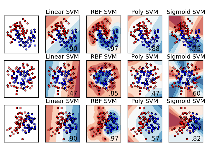
Look closely at the results:

• Top Row (Moons): The Linear SVM struggles. The RBF SVM creates a near-perfect boundary. The Polynomial SVM also finds a curved boundary but is less effective than RBF.
• Middle Row (Circles): This is a classic non-linear problem. The Linear and Polynomial SVMs fail completely, achieving an accuracy no better than random guessing. The RBF SVM, however, easily learns the circular boundary.
• Bottom Row: This is another complex boundary. Again, the RBF kernel proves to be the most flexible and effective.

This visual evidence highlights a key takeaway: the RBF kernel is an excellent default choice for SVMs when you don't have prior knowledge about your data's structure, due to its ability to handle a wide variety of non-linear patterns.

For a final summary, let's look at a clear comparison between the linear and non-linear approaches.

Conclusion

In this lesson, you've unlocked the true power of Support Vector Machines by understanding the kernel trick. You've moved beyond simple linear boundaries and can now see how SVMs tackle complex, real-world classification tasks.

Key Takeaways:

• When data is not linearly separable, SVMs can project it into a higher-dimensional space where a separating hyperplane might exist.
• The kernel trick is a highly efficient method that computes the relationships (dot products) between points in this high-dimensional space without ever explicitly performing the costly transformation.
• The Polynomial kernel creates polynomial decision boundaries, with the degree hyperparameter controlling complexity.
• The RBF kernel is a powerful, general-purpose kernel that can create highly complex boundaries. Its gamma hyperparameter controls the influence of individual data points, managing the tradeoff between a smooth and a complex decision boundary.
• The choice of kernel and its hyperparameters is critical for the SVM's performance and depends on the underlying structure of the data.

In our next lesson, we will step back and evaluate the SVM algorithm as a whole. Now that you understand both its linear and non-linear capabilities, we will discuss its primary strengths and weaknesses, its sensitivity to things like feature scaling, and when you should choose it over other models like Logistic Regression or Random Forests.