Understanding Linear Regression: Intuition, Cost Function, and Assumptions

Modeling Relationships with a Line

At its heart, linear regression is a statistical method for modeling the relationship between a dependent variable (the target you want to predict) and one or more independent variables (the features). The "linear" part of the name signifies that the model assumes this relationship can be represented by a straight line.

For the simple case of one feature (X) and one target (Y), this relationship is described by the familiar equation of a line:

Let's break this down:

• $Y$ is the dependent variable (the target).
• $X$ is the independent variable (the feature).
• ${\beta }_0$ is the intercept, representing the predicted value of $Y$ when $X$ is zero.
• ${\beta }_1$ is the slope or coefficient for feature $X$. It quantifies the change in $Y$ for a one-unit change in $X$.
• $ϵ$ is the error term, which captures the variability in $Y$ that cannot be explained by the linear relationship with $X$.

The goal of a linear regression model is to learn the optimal values for the coefficients (${\beta }_0$ and ${\beta }_1$) from the training data. But how does it determine what is "optimal"?

Finding the Best Line: Ordinary Least Squares (OLS)

Imagine scattering your data points on a plot. You could draw an infinite number of straight lines through them. The "best" line is the one that comes closest to all the data points simultaneously. To quantify this, we first need to define the error.

For each data point, the error, or residual, is the vertical distance between the actual value ($Y_i$) and the value predicted by the line (${\hat{Y}}_i$).

We can't simply sum these residuals, because positive errors (when the line is below the point) and negative errors (when the line is above) would cancel each other out. To solve this, we square each residual. This makes all errors positive and has the added benefit of penalizing larger errors much more heavily than smaller ones.

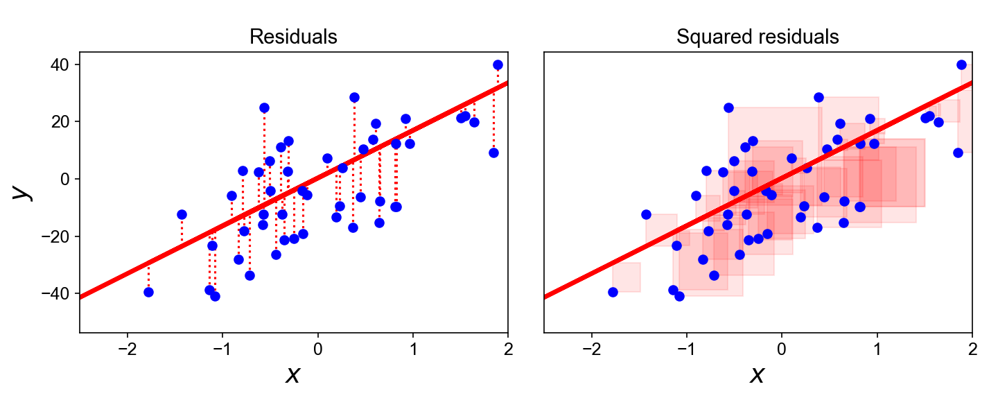
The sum of all these squared residuals is called the Sum of Squared Errors (SSE) or Residual Sum of Squares (RSS). Dividing this by the number of data points gives us the Mean Squared Error (MSE), which is the most common cost function for regression problems.

The method used to find the line that minimizes this cost function is called Ordinary Least Squares (OLS). The following video provides a wonderfully clear, intuitive explanation of this process.

As you saw, OLS systematically finds the unique line that minimizes the sum of the squared vertical distances from the data points to that line. While there is a direct analytical formula to solve for the coefficients in OLS (known as the normal equation), understanding it as an optimization problem—finding the parameters that minimize a cost function—is a crucial concept that applies to nearly all machine learning models.

For a more detailed textual summary of these concepts, the following resource provides a concise walkthrough.

The Rules of the Game: Key Assumptions

For the coefficients estimated by OLS to be reliable, unbiased, and efficient, several key assumptions about the data and the residuals must be met. Violating these assumptions doesn't necessarily mean the model is useless, but it can make your interpretations and conclusions misleading.

These assumptions can be easily remembered with the acronym LINE:

• Linearity
• Independence
• Normality
• Equal variance (Homoscedasticity)

The following video provides a clear, practical explanation of each assumption, why it matters, and how to spot violations. This is a very common topic in data science interviews, so a solid grasp here is valuable.

To complement the video, you can refer to the "Regression Cookbook" resource again for a more technical description of how to check these assumptions, often involving specific statistical tests that you may encounter in your coursework.

Conclusion

In this lesson, we have laid the groundwork for our study of supervised learning by understanding linear regression. You've learned how this model conceptualizes the relationship between variables as a line, how it defines the "best" line by minimizing the Mean Squared Error, and the OLS method used to achieve this. Crucially, you now also understand the four key assumptions (LINE) that must be checked to ensure the model's results are valid and interpretable.

Key Takeaways:

• Linear Regression models a linear relationship between features and a target variable.
• The cost function, typically Mean Squared Error (MSE), quantifies how poorly the model fits the data.
• Ordinary Least Squares (OLS) is the optimization method that finds the model parameters (coefficients) that minimize the MSE.
• The reliability of a linear regression model depends on four key assumptions, remembered by the acronym LINE: Linearity, Independence, Normality, and Equal variance.

In this lesson, we discussed that OLS finds the optimal parameters by minimizing the cost function. For linear regression, there is a direct analytical solution to this problem. However, for most other machine learning algorithms, no such direct solution exists. Instead, we must use an iterative optimization algorithm to gradually "descend" towards the minimum of the cost function. In our next lesson, we will explore the most fundamental and important of these algorithms: Gradient Descent.