Gradient Descent: Optimizing Machine Learning Models

The Core Idea: Descending the Cost Function

Imagine you are a hiker on a mountain in a thick fog. Your goal is to get to the lowest point in the valley, but you can only see the ground a few feet around you. What's your strategy? A sensible approach would be to feel the slope of the ground where you are standing and take a step in the steepest downhill direction. You would repeat this process—sense the slope, take a step—until you reach a point where the ground is flat, indicating you've arrived at the bottom of a valley.

This is precisely the intuition behind gradient descent.

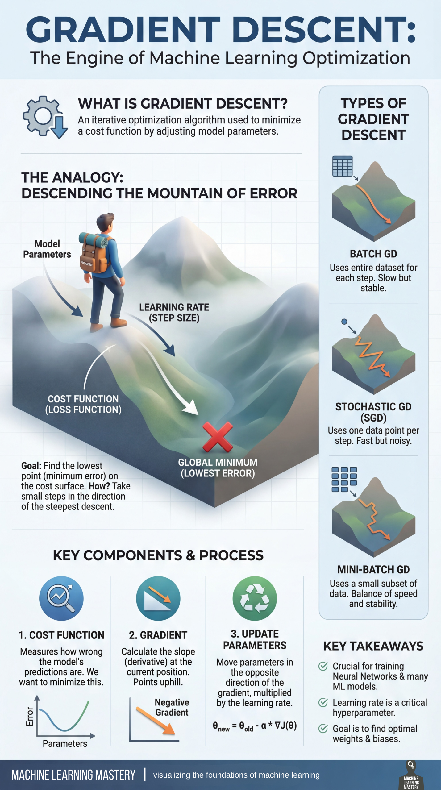
Let's translate this analogy into the context of machine learning:

• The Hiker's Position: This represents the current values of our model's parameters (e.g., the intercept ${\theta }_0$ and slope ${\theta }_1$ in linear regression).
• The Mountain Landscape: This is the cost function (like MSE), visualized as a surface where the height at any point is the cost for a given set of parameters. Our goal is to find the parameter values that correspond to the lowest point on this surface.
• The Steepest Direction: In calculus, the gradient of a function at a particular point is a vector that points in the direction of the steepest ascent. To go downhill, we simply move in the opposite direction of the gradient.
• The Step Size: How large of a step should the hiker take? This is controlled by a crucial hyperparameter called the learning rate.

The StatQuest video below provides an exceptionally clear, step-by-step walkthrough of this entire process. It starts by optimizing a single parameter and then extends the logic to two, perfectly building the intuition from the ground up.

The Gradient Descent Algorithm

As you saw in the video, gradient descent is an iterative process. Let's formalize the key update rule. If $J(\vec{\theta })$ is our cost function, which depends on a vector of parameters $\vec{\theta }$, the update at each step $t$ is:

Let's break this down:

• ${\vec{\theta }}^{(t+1)}$ is the new set of parameters we are calculating.
• ${\vec{\theta }}^{(t)}$ is our current set of parameters.
• $\alpha$ is the learning rate, a small positive number (e.g., 0.01) that controls the step size.
• ${\nabla }_{\vec{\theta }}J({\vec{\theta }}^{(t)})$ is the gradient of the cost function with respect to the parameters at our current position. This vector points in the direction of the steepest increase in cost.

By subtracting the scaled gradient ($\alpha \nabla J$), we are nudging the parameters in the direction that most rapidly decreases the cost. We repeat this process until the algorithm converges. Convergence typically occurs when the gradient becomes very close to zero (we're at the bottom of a valley) or after a predefined number of iterations.

The following text provides a solid summary of this process, moving from a single-dimension function to the multi-dimensional case.

Visualizing the Gradient in High Dimensions

For functions with one or two parameters, we can visualize the cost surface. But what about a complex model with thousands or even millions of parameters? While we can't draw a picture, the logic remains identical. The gradient is a high-dimensional vector, and the algorithm simply takes a small step in the direction opposite to this vector.

The 3Blue1Brown video below offers a superb visual intuition for how to think about the gradient in this high-dimensional context.

The Three Flavors of Gradient Descent

A critical detail in applying gradient descent is deciding how much data to use when calculating the gradient at each step. This choice gives rise to three common variants of the algorithm.

1. Batch Gradient Descent: In each step, the gradient is calculated using the entire training dataset.

   • Pros: Provides a very accurate estimate of the gradient, leading to a smooth, direct path towards the minimum.
   • Cons: Computationally very expensive and slow, especially for large datasets, as it requires processing every single data point for just one update.

2. Stochastic Gradient Descent (SGD): In each step, the gradient is calculated using only one randomly selected data point from the training set.

   • Pros: Extremely fast per-step updates. The noisy updates can also help the algorithm jump out of shallow local minima.
   • Cons: The path to the minimum is very erratic and noisy. It doesn't move directly towards the minimum but zig-zags around it.

3. Mini-Batch Gradient Descent: This is the most common and practical approach. In each step, the gradient is calculated on a small, random subset of the data, called a "mini-batch" (e.g., 32, 64, or 256 data points).

   • Pros: Strikes a balance between the accuracy of Batch GD and the speed of SGD. It provides a good-enough gradient estimate for a stable convergence path while being computationally efficient.
   • Cons: Introduces a new hyperparameter: the batch size.

The following resource provides a clear distinction between these methods.

A Note on Convexity and Advanced Optimizers

One important property of a cost function is convexity. A convex function has a single "bowl" shape, meaning it has only one minimum—a global minimum. The MSE cost function for linear regression is convex. For convex problems, gradient descent is guaranteed to find the global minimum.

However, many cost functions for advanced models (like neural networks) are non-convex, with many "valleys" or local minima. In these cases, gradient descent may converge to a local minimum, which might not be the best possible solution. The noisy nature of SGD and Mini-Batch GD can sometimes help escape poor local minima.

Finally, it's worth knowing that the "vanilla" gradient descent we've discussed has evolved. Modern deep learning relies on more advanced optimizers like Adam, RMSprop, and others that incorporate concepts like momentum (to accelerate through valleys) and adaptive learning rates (adjusting the step size for each parameter). While the details are beyond this lesson, they all build on the fundamental principles of gradient descent you've learned here.

Conclusion

In this lesson, you've learned about gradient descent, the workhorse optimization algorithm of modern machine learning. It provides a general, iterative framework for finding the model parameters that minimize a cost function, even when a direct analytical solution like OLS is not available.

Key Takeaways:

• Gradient Descent is an iterative optimization algorithm that minimizes a cost function by repeatedly taking steps in the direction opposite to the gradient.
• The gradient is a vector of partial derivatives that points in the direction of the steepest ascent of the cost function.
• The learning rate ($\alpha$) is a critical hyperparameter that controls the step size. It must be tuned carefully to ensure convergence.
• Batch, Mini-Batch, and Stochastic gradient descent are variants that trade off computational cost and update accuracy. Mini-Batch is the most common approach.
• For convex cost functions, gradient descent is guaranteed to find the global minimum. For non-convex functions, it finds a local minimum.

Now that we have established two methods for fitting a linear regression model (OLS and Gradient Descent), our next step is to learn how to quantitatively measure how well our model performs. In the next lesson, we will dive into the key metrics used to evaluate regression models, such as MSE, RMSE, MAE, and R-squared.