Evaluating Regression Models with Key Metrics

Welcome to our next lesson. In our previous sessions, we focused on the mechanics of fitting a linear regression model. You learned about solving for model parameters directly with Ordinary Least Squares and iteratively with Gradient Descent. Now that we know how to build a model, we need to answer a critical question: "How good is it?" This lesson is dedicated to the essential metrics used to evaluate the performance of regression models.

We will explore four fundamental metrics: Mean Absolute Error (MAE), Mean Squared Error (MSE), Root Mean Squared Error (RMSE), and the R-squared ( $R^{2}$ ) score. Each metric provides a different perspective on your model's accuracy, and understanding their nuances is crucial for both optimizing models and communicating their performance effectively.

Measuring Prediction Error

At the heart of regression evaluation is the concept of error, or a residual. For any single data point, the error is simply the difference between the actual value ( $y_{i}$ ) and the value predicted by your model ( $y^_{i}$ ).

error_{i} = y_{i} - y^_{i}

Our goal is to aggregate these individual errors across the entire dataset into a single, meaningful score. Let's examine the most common ways to do this.

Mean Absolute Error (MAE)

The most straightforward approach is to take the average of the absolute values of the errors. This is the Mean Absolute Error (MAE).

MAE = \frac{1}{n} i = 1 \sum n ∣ y_{i} - y^_{i} ∣

Intuition: The MAE answers the question: "On average, how far were our model's predictions from the actual values?"

Interpretability: Its primary advantage is its simplicity. If the MAE of a house price prediction model is $15,000, it means the model's predictions are, on average, off by $15,000. The error is in the same unit as the target variable, making it easy to explain.
Outlier Robustness: Because it doesn't square the errors, a few large errors (outliers) will not dominate the metric. It treats a $20,000 error as being exactly twice as bad as a $10,000 error.

Mean Squared Error (MSE)

You're already familiar with Mean Squared Error (MSE); it's the cost function we minimized in our previous lessons on OLS and gradient descent.

MSE = \frac{1}{n} i = 1 \sum n (y_{i} - y^_{i})^{2}

Intuition: The MSE is designed to heavily penalize larger errors.

Outlier Sensitivity: By squaring the error term, MSE gives much more weight to large mistakes. An error of 10 results in a squared error of 100, while an error of 100 results in a squared error of 10,000. This is useful when large errors are particularly undesirable.
Optimization-Friendly: The MSE is a differentiable function, which, as you know from our gradient descent lesson, makes it well-suited for use as a loss function during model training.
Lack of Interpretability: A major drawback is that the final value is in squared units (e.g., "squared dollars"). This makes it difficult to interpret in the context of the original problem.

Root Mean Squared Error (RMSE)

The Root Mean Squared Error (RMSE) is the square root of the MSE. It was developed to address the interpretability issue of MSE.

RMSE = \frac{1}{n} i = 1 \sum n (y_{i} - y^_{i})^{2}

Intuition: RMSE represents the standard deviation of the prediction errors (residuals).

Interpretability: Like MAE, RMSE is in the same unit as the target variable, making it easier to understand. An RMSE of $20,000 for our house price model means the typical deviation of our predictions from the actual prices is $20,000.
Outlier Sensitivity: Because it's based on MSE, it retains the property of being sensitive to large errors. RMSE will always be greater than or equal to MAE, with the difference being larger when there are larger individual errors.

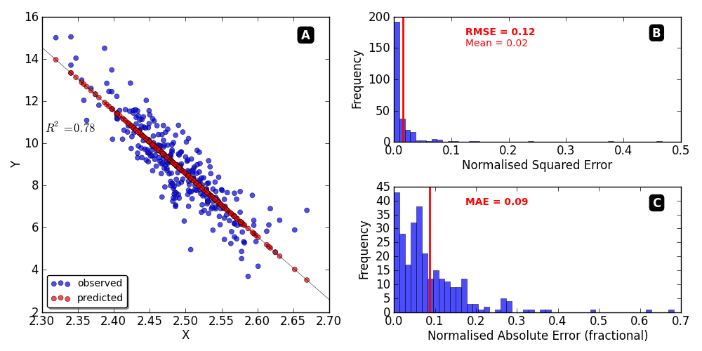
The following image provides a clear visual summary of the difference in how MSE and MAE handle errors.

This diagram illustrates how Mean Squared Error (MSE) heavily penalizes larger errors (outliers) due to the squaring operation, while Mean Absolute Error (MAE) treats errors linearly, making it more robust to outliers.

The image below shows a real example. Panel A is a scatter plot of predicted vs. observed values. Panels B and C show the distribution of the normalized squared errors and absolute errors, respectively. Notice how the RMSE value is larger than the MAE value, reflecting the influence of the larger errors present in the data.

Panel A shows a regression fit. Panel B is a histogram of squared errors, used to calculate RMSE. Panel C is a histogram of absolute errors, used for MAE. The red lines indicate the mean of these distributions.

The following video provides an excellent summary of all the metrics we will discuss, explaining their formulas, trade-offs, and when to use them.

Evaluation Metrics For Regression - When & Why To Use What

This video, "Evaluation Metrics For Regression," gives a concise and practical overview of the key metrics.

Start by watching the segment on MSE and RMSE, from this timestamp. It clearly explains the formulas and the primary difference between them: optimization utility (MSE) vs. human interpretability (RMSE). Next, watch the explanation of MAE from this section. The presenter gives a great intuitive hook: MAE tells you "on average, how wrong is my prediction?"

Measuring Goodness-of-Fit: R-Squared ( $R^{2}$ )

While MAE, MSE, and RMSE quantify the magnitude of the error, R-squared ( $R^{2}$ ), also called the coefficient of determination, answers a different question: "How much of the variation in the target variable can be explained by our model?"

It provides a relative measure of fit. It compares your model's performance to that of a naive baseline model that simply predicts the mean of the target variable ( $y ˉ$ ) for every data point.

The formula is:

R^2 = 1 - \frac{\text{Sum of Squared Residuals (SS_res)}}{\text{Total Sum of Squares (SS_tot)}} = 1 - \frac{\sum (y_i - \hat{y}_i)^2}{\sum (y_i - \bar{y})^2}

$S S_{r es}$ : This is the sum of squared errors from your model. It quantifies the variation that your model cannot explain.
$S S_{t o t}$ : This is the sum of squared errors from the naive mean model. It represents the total variation in the data.

Interpretation:

An $R^{2}$ of 1.0 indicates a perfect fit, where the model explains all the variance in the data.
An $R^{2}$ of 0.0 indicates that your model is no better than the baseline model that just predicts the mean.
A negative $R^{2}$ indicates that your model is even worse than the baseline mean model.
An $R^{2}$ of 0.75 means your model explains 75% of the variance in the target variable.

A Caveat: Adjusted R-Squared

A known issue with $R^{2}$ is that it will never decrease when you add new features to your model, even if those features are completely irrelevant. This can be misleading. To counter this, the Adjusted $R^{2}$ was created. It modifies the $R^{2}$ formula to penalize the score for each additional feature added. A higher adjusted $R^{2}$ implies a better model that is not overly complex.

The following resource gives a good overview of all these metrics.

Evaluation Metrics for Your Regression Model

This article from Analytics Vidhya provides a clear, written explanation of each metric we've discussed.

Read through the sections explaining Mean Absolute Error (MAE), Mean Squared Error (MSE), Root Mean Squared Error (RMSE), and both R Squared and Adjusted R Squared. Focus on understanding the core intuition, advantages, and disadvantages of each.

How to Choose the Right Metric?

The choice of metric depends on your business goal and the data's characteristics, especially the presence of outliers.

RMSE vs. MAE: This is the most common trade-off.
- Choose RMSE if you want to heavily penalize large errors. For example, in financial forecasting, a very large error could be catastrophic, so you want a metric that highlights these.
- Choose MAE if you want a metric that is more robust to outliers and represents the average error magnitude. If a model is off by $100K, and another is off by $200K, MAE sees the second error as twice as bad. RMSE sees it as four times as bad.
R-Squared: Use this to communicate the overall "explanatory power" of your model in a context-independent way. An $R^{2}$ of 0.8 is generally strong, regardless of whether the target is house prices in dollars or sensor readings in volts.
Error Metrics (MAE, RMSE) vs. R-Squared: Use error metrics when you need to know the prediction error in absolute, tangible units. Use R-squared when you want a normalized score of how well the model fits the data. In practice, you should always report both.

The following resource does an excellent job of demonstrating these trade-offs with practical code examples.

Regression Model Scoring with Scikit-Learn

This article demonstrates how different metrics behave, particularly in the presence of outliers.

Read the section on Mean Absolute Error (MAE) to understand its linear treatment of error. Next, read the section on Mean Squared Error (MSE) to see how squaring affects the score. Finally, review the Conclusion's first trade-off. The simple code examples there perfectly illustrate how MSE's score explodes with an outlier compared to MAE's score.

Conclusion

You have now learned how to measure the performance of your regression models. This is a critical step in the machine learning workflow, allowing you to compare different models and tune their parameters.

Key Takeaways:

MAE (Mean Absolute Error): Gives the average absolute error in the original units. It's robust to outliers.
MSE (Mean Squared Error): A common loss function for optimization. It's in squared units and heavily penalizes large errors.
RMSE (Root Mean Squared Error): A compromise that is sensitive to large errors like MSE but is in the original units like MAE, making it interpretable.
R-Squared ( $R^{2}$ ): Measures the proportion of variance in the target variable that is explained by the model, providing a context-independent measure of fit.

So far, we've evaluated our model's performance on a single train-test split. But what if that split was lucky (or unlucky)? To get a more reliable and robust estimate of our model's true performance on unseen data, we need a more rigorous validation strategy. In our next lesson, we will explore k-fold cross-validation, a powerful technique for achieving just that.

Recommended resources