ROC Curves and AUC Calculation

From Thresholds to a Curve

In the previous lesson, the central idea was that a logistic regression model outputs probabilities, and we apply a threshold (like 0.5) to make a binary classification. The ROC curve is generated by plotting the model's performance at every conceivable threshold, not just one.

The best way to build intuition for this is to see it constructed step-by-step. The following video from StatQuest does an exceptional job of this.

As you just saw, an ROC curve is a two-dimensional plot with two key rates on its axes:

• Y-axis: True Positive Rate (TPR). This is the exact same metric as Recall or Sensitivity, which you already know. It answers: Of all the actual positive instances, what fraction did the model correctly identify?
  $\text{TPR}=\text{Recall}=\frac{TP}{TP+FN}$

• X-axis: False Positive Rate (FPR). This metric might be new. It answers: Of all the actual negative instances, what fraction did the model incorrectly classify as positive?
  $\text{FPR}=\frac{FP}{FP+TN}$

The ROC curve visualizes the tradeoff between these two metrics. As you lower the classification threshold to capture more true positives (increasing TPR), you inevitably also misclassify more negatives as positive (increasing FPR).

Interpreting the ROC Curve and AUC

Now that you understand how an ROC curve is built, let's focus on how to interpret it. A model's curve tells a story about its ability to separate the positive and negative classes.

As the reading highlights, we can summarize the interpretation as follows:

• Random Guess Line: The diagonal line from (0,0) to (1,1) represents a classifier with no predictive power—it's equivalent to random guessing. A model whose curve falls on this line has a TPR equal to its FPR.
• Perfect Classifier: The point (0,1) represents a perfect classifier: it achieves a 100% True Positive Rate with a 0% False Positive Rate. An effective model will have a curve that "bows" up towards this top-left corner.
• Model Comparison: The closer a curve follows the top-left border of the plot, the better the model. If you are comparing two models, the one whose curve is consistently higher and to the left is superior.

While visually comparing curves is useful, it's often more practical to summarize a curve's performance with a single number. This is the Area Under the (ROC) Curve, or AUC.

The AUC score has a range:

• AUC = 1.0: A perfect classifier.
• AUC = 0.5: A classifier with no predictive value (same as random guessing).
• AUC < 0.5: A classifier that is worse than random guessing. (This is rare; it often indicates a bug or that the model's predictions are inverted).

A powerful and intuitive way to understand AUC is through its probabilistic interpretation.

As you've just read, the AUC has a wonderfully elegant meaning:

AUC is the probability that the model will rank a randomly chosen positive instance higher than a randomly chosen negative instance.

An AUC of 0.85 means that if you pick one random positive example and one random negative example, there is an 85% chance that your model assigned a higher probability score to the positive example. This interpretation makes AUC a measure of how well the model separates the two classes.

ROC and AUC in Python

Given your background, you'll find implementing this in scikit-learn very direct. The sklearn.metrics module provides all the necessary functions.

It's crucial to remember that to generate a smooth, accurate ROC curve, you must use the predicted probabilities from your model, not the final 0/1 classifications.

Here is a summary of the key functions you will use from sklearn.metrics:

1. roc_curve(y_true, y_probabilities): This function computes the TPR and FPR for various thresholds. It returns three arrays: fpr, tpr, and thresholds.
2. roc_auc_score(y_true, y_probabilities): This function directly computes the Area Under the Curve.
3. RocCurveDisplay.from_estimator(model, X_test, y_test) or RocCurveDisplay.from_predictions(y_test, y_probabilities): These are convenient plotting functions that handle the roc_curve calculation and plotting with matplotlib in one step.

Here is a typical implementation pattern:

from sklearn.datasets import make_classification
from sklearn.model_selection import train_test_split
from sklearn.linear_model import LogisticRegression
from sklearn.metrics import roc_curve, roc_auc_score, RocCurveDisplay
import matplotlib.pyplot as plt




# Generate data and train a model
X, y = make_classification(n_samples=1000, n_features=10, random_state=42)
X_train, X_test, y_train, y_test = train_test_split(X, y, test_size=0.2, random_state=42)

model = LogisticRegression()
model.fit(X_train, y_train)




# Get predicted probabilities for the positive class
y_probs = model.predict_proba(X_test)[:, 1]




# 1. Calculate AUC
auc = roc_auc_score(y_test, y_probs)
print(f'AUC: {auc:.4f}')




# 2. Get the ROC curve points
fpr, tpr, thresholds = roc_curve(y_test, y_probs)




# 3. Plotting with RocCurveDisplay (the easy way)
RocCurveDisplay.from_predictions(y_test, y_probs)
plt.plot([0, 1], [0, 1], 'k--', label='Random Guess') # Add the random guess line
plt.title('ROC Curve')
plt.show()

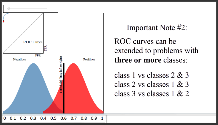
Finally, this concept can be extended to multi-class problems, typically by using a "one-vs-rest" (OvR) approach, where you plot a separate ROC curve for each class against all other classes.

Conclusion

You have now added the final, essential visualization and metric to your classification evaluation toolkit. You can now assess a model not just at a single point, but across its entire operational range.

Key Takeaways:

• The ROC curve plots the True Positive Rate (Recall) against the False Positive Rate at all possible classification thresholds.
• An effective model's curve bows towards the top-left corner (TPR=1, FPR=0), while a random model follows the diagonal line.
• The Area Under the Curve (AUC) quantifies the model's overall ability to discriminate between positive and negative classes into a single value between 0.5 and 1.0.
• Intuitively, AUC represents the probability that the model will assign a higher score to a randomly chosen positive instance than to a randomly chosen negative one.
• In scikit-learn, always use the output of predict_proba() to generate smooth and meaningful ROC curves.

In our next lesson, we will synthesize everything from this module. You will apply logistic regression to a real-world binary classification problem and perform a comprehensive evaluation using the confusion matrix, precision, recall, F1-score, and now, ROC/AUC. We will also formally discuss how to extend logistic regression to multi-class scenarios.