Logistic Regression for Binary Classification

A Complete Workflow: From Data to Evaluation

We will build a model to predict whether a breast cancer tumor is malignant or benign based on various cell measurements. This is a classic binary classification problem where the stakes are high, making a nuanced evaluation of the model's errors particularly important.

The GeeksForGeeks article, "Logistic Regression using Python," provides an exceptionally clear, step-by-step guide for this exact task. We will follow its structure to load the data, preprocess it, train our model, and evaluate its performance.

Let's summarize the setup process you just reviewed. The standard workflow is:

1. Load Data: Bring the dataset into our environment.
2. Separate X and y: Isolate the features (X) from the target variable (y).
3. Split Data: Divide X and y into training and testing sets. This is crucial to ensure we evaluate the model on data it has never seen before.
4. Scale Features: Standardize the feature values. We fit the scaler only on the training data (X_train) and then use that same fitted scaler to transform both the training and testing data (X_train and X_test). This prevents information from the test set from "leaking" into the training process.

Training the Model and Making Predictions

With our data prepared and split, the next steps are to train the logistic regression model and use it to make predictions on our held-out test set.

As you saw, the process in scikit-learn is remarkably direct:

1. Instantiate: model = LogisticRegression() creates an instance of the model.
2. Train: model.fit(X_train, y_train) trains the model by finding the optimal coefficients for the features in X_train to predict y_train.
3. Predict: y_pred = model.predict(X_test) uses the trained model to generate class labels (0 or 1) for the unseen test data.

To perform a complete evaluation, especially for plotting the ROC curve, we also need the predicted probabilities. We can get these using:

# Probabilities for the positive class (e.g., 'malignant')
y_probabilities = model.predict_proba(X_test)[:, 1] 

Evaluating Model Performance: A Multi-Faceted Approach

Now comes the most critical part: evaluating our model's performance. A single metric like accuracy can be misleading, especially with imbalanced datasets. Therefore, we will use the full suite of metrics we've learned.

The Confusion Matrix

The confusion matrix is the foundation of classification evaluation, giving us a raw count of correct and incorrect predictions.

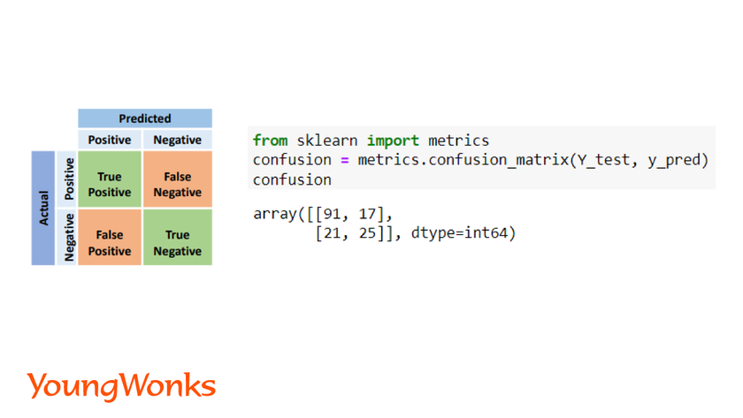
Let's look at the specific metrics derived from the matrix. The GeeksForGeeks article provides a fantastic, code-driven overview of this entire evaluation process.

Let's digest the results from the article and interpret them in the context of our cancer prediction problem.

• Confusion Matrix:

  • True Positives (TP): The model correctly identified a tumor as malignant.
  • True Negatives (TN): The model correctly identified a tumor as benign.
  • False Positives (FP) (Type I Error): The model incorrectly classified a benign tumor as malignant. This would cause unnecessary stress and further testing for the patient.
  • False Negatives (FN) (Type II Error): The model incorrectly classified a malignant tumor as benign. This is the most dangerous error, as a patient with cancer might be told they are healthy, delaying critical treatment.

• Precision, Recall, and F1-Score: The classification_report in scikit-learn provides these metrics.

  • Recall (Sensitivity or TPR): For the "malignant" class, this answers: "Of all the patients who truly had a malignant tumor, what percentage did our model correctly identify?" In a medical context, we want this to be as high as possible to minimize false negatives.
  • Precision: For the "malignant" class, this answers: "Of all the patients our model flagged as having a malignant tumor, what percentage actually did?" High precision reduces the number of false alarms (false positives).
  • F1-Score: The harmonic mean of precision and recall, providing a single score that balances both concerns.

• ROC Curve and AUC:

  • The ROC curve visualizes the trade-off between the True Positive Rate (Recall) and the False Positive Rate across all possible thresholds.
  • The AUC score gives us a single number summarizing the model's ability to distinguish between the two classes. An AUC of 0.98, as seen in the article, indicates an excellent ability to separate malignant from benign cases. It means there is a 98% chance that the model will assign a higher probability score to a randomly chosen malignant tumor than to a randomly chosen benign one.

Alternative Walkthrough: The Pima Diabetes Dataset

The workflow we just followed is highly generalizable. To prove this, you can review another excellent tutorial from DataCamp that applies the exact same principles to a different medical dataset: predicting diabetes.

Conclusion

In this lesson, you have consolidated all the theoretical concepts from this module into a single, practical workflow. You have successfully trained a logistic regression classifier on a real-world dataset and, more importantly, performed a robust evaluation using a complete set of metrics.

Key Takeaways:

• A standard machine learning workflow for classification involves data preprocessing (scaling), train-test splitting, model training, and prediction.
• Evaluating a classification model requires a suite of metrics, not just accuracy.
• The confusion matrix provides the raw data for evaluation, breaking down predictions into TP, TN, FP, and FN.
• Precision and Recall measure different aspects of a model's performance, and the context of the problem (e.g., the cost of false negatives in medical diagnosis) dictates which is more important.
• The ROC curve and AUC provide a threshold-independent measure of your model's ability to discriminate between classes.

We have focused exclusively on binary classification. In our next lesson, we will explore how logistic regression can be extended to handle problems with more than two classes, using strategies like One-vs-Rest (OvR) and the softmax function.