Welcome back! In our last lesson, we delved into the theory behind Principal Component Analysis, understanding it as a method for finding new, uncorrelated features (principal components) that maximize the variance of your data. We established the connection between these components and the eigenvectors of the data's covariance matrix.
Today, we transition from theory to practice. This lesson is all about applying PCA to a real, high-dimensional dataset using Python and scikit-learn. Our primary focus will be on answering the most critical practical question when using PCA: "How many components should I keep?" You will learn how to use the concept of "explained variance" to make an informed decision, ensuring you reduce dimensionality while retaining the essential information in your data.
The PCA Workflow with scikit-learn
As you know from your experience with Python's data science libraries, scikit-learn offers a consistent and intuitive API. The PCA workflow is no different and generally involves three main steps:
- Scale the data: PCA is sensitive to the scale of features. As we discussed previously, its goal is to maximize variance, so features with larger scales can disproportionately influence the principal components. Therefore, using
StandardScaleris a crucial prerequisite. - Instantiate and fit the PCA model: Create a
PCAobject and use its.fit()method on the scaled data. This step computes the principal components (eigenvectors) and their corresponding explained variance (eigenvalues). - Transform the data: Use the
.transform()method to project the original data onto the chosen principal components, creating the new, lower-dimensional representation.
Josh Starmer's StatQuest video provides a clear, code-along demonstration of this process.
This video walks through the practical steps of applying PCA in Python, from scaling the data to fitting the model and transforming the data into its principal components.
Watch the following segments to see the standard workflow in action: Centering and Scaling (watch here): Pay attention to the emphasis on scaling the data before performing PCA. The video uses a dataset where samples are columns, requiring a transpose (.T), which is common in bioinformatics. In many other contexts, your samples will already be in rows. Fitting and Transforming (watch here): This part shows how to create a PCA object and then use the .fit() and .transform() methods. Notice the object-oriented approach: the pca object is first "trained" (fitted) on the data to learn the components, and can then be used to transform data.
Explained Variance: The Key to Choosing Components
In the last lesson, we learned that the eigenvalues of the covariance matrix measure the amount of variance captured by each corresponding eigenvector (principal component). When using scikit-learn, we don't have to calculate these ourselves. The fitted PCA object stores this information in a very convenient attribute: explained_variance_ratio_.
This attribute returns an array where each value is the percentage of the total dataset variance captured by the corresponding principal component. Because PCA orders the components by the variance they explain, the first value in this array will be the largest, the second will be the next largest, and so on.
The two plots below illustrate this concept perfectly.
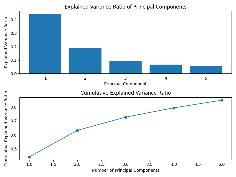
Our goal is to keep the fewest components that explain the most variance. But how do we decide the cutoff?
How to Choose the Number of Components
There are a few standard methods for choosing the optimal number of components to retain. Let's explore the most common ones.
1. The Cumulative Explained Variance Threshold
The most widely used method is to set a threshold for the total amount of variance you wish to preserve. A common practice is to aim for a value between 90% and 99%. You can then plot the cumulative explained variance and see how many components are required to cross this threshold.
The plot below demonstrates this. To explain 80% of the variance in this particular dataset, we would need to keep approximately 60 principal components.

2. The Scree Plot and Elbow Method
Another popular approach uses the scree plot we saw earlier (a bar chart of the explained variance per component). With this method, you look for an "elbow" or "knee" in the plot—a point where the variance explained by subsequent components drops off and the line begins to flatten. The components up to this elbow are considered the most significant.
The following video demonstrates how to create a scree plot and use both the elbow method and another heuristic called Kaiser's Rule.
Principal Component Analysis in Python | How to Apply PCA | Scree Plot, Biplot, Elbow & Kaisers Rule
This video provides a detailed guide on using variance information to decide the ideal number of components. It covers the scree plot, the elbow method, and Kaiser's rule.
Please watch the segment from Explained Variance to Component Selection. Focus on how the explained_variance_ratio_ is used to create the scree plot. The narrator then explains two key decision techniques: Elbow Method: Find the point on the scree plot where the curve bends, suggesting diminishing returns from adding more components. Kaiser's Rule: Keep only the components whose explained variance is greater than 1 (when using the non-normalized explained_variance_ attribute). This essentially means keeping components that explain more variance than a single original variable would on average.
3. The scikit-learn Shortcut
scikit-learn provides a wonderfully convenient way to implement the cumulative variance threshold method directly. Instead of providing an integer for the n_components parameter, you can provide a float between 0.0 and 1.0. For instance, PCA(n_components=0.95) will automatically select the minimum number of components required to preserve 95% of the variance.
A Practical Walkthrough
Let's put all this together by walking through a complete example. The following reading uses the scikit-learn wine dataset, which has 13 features. You will apply PCA and use the methods we've just discussed to choose the number of components.
Practical Intro to Principal Components Analysis for Dimension ...
This article provides a step-by-step Python implementation of PCA, demonstrating the full workflow from data loading to component selection.
Please read through the following sections of the article: Loading and Scaling the Data: Start by reading from the beginning of Section 2. This covers loading the wine dataset and, importantly, applying StandardScaler. Applying PCA: Continue with the section on Applying PCA. This shows the basic instantiation and transformation using scikit-learn. Explained Variance Ratio: Now, read the short section on the Explained Variance Ratio. This shows you how to access the .explained_variance_ratio_ attribute. A quick note: The author gets a strange result of [0.998, 0.0017] because they accidentally applied PCA to the unscaled data in one step. One feature (proline) has a variance thousands of times larger than the others, so the first principal component almost exclusively captures that single feature. This is a perfect example of why we must always scale our data before using PCA. The author corrects this in the next step. Choosing the Number of Components: This is the most important part. Read the section titled Choosing Number of Components. It demonstrates two methods: First, it shows the code to generate the cumulative explained variance plot, which is the visual tool for the threshold and elbow methods. Second, it demonstrates the scikit-learn shortcut by initializing PCA(n_components=0.96) and shows that it automatically selects the correct number of components (10, in this case).
Conclusion
In this lesson, you have bridged the gap between the theory of PCA and its practical implementation. You now have a robust workflow for applying PCA and, most importantly, several well-defined methods for selecting the right number of components to retain.
Key Takeaways:
- PCA Workflow: The standard process in
scikit-learnis to scale the data, fit aPCAobject to it, and then transform the data into its new, lower-dimensional form. - Explained Variance is Key: The
explained_variance_ratio_attribute is the cornerstone of component selection. It tells you what percentage of the total information is captured by each component. - Component Selection Methods:
- Cumulative Variance Plot: Plot the cumulative sum of explained variance and choose the number of components that exceeds a desired threshold (e.g., 95%).
- Scree Plot & Elbow Method: Look for the "elbow" in the plot of individual component variances to find the point of diminishing returns.
scikit-learnShortcut: Simply pass a float (e.g.,0.95) to then_componentsparameter to havescikit-learnselect the components for you.
What's Next:
You've learned how to reduce the dimensionality of your data while preserving most of its informational content. In the next lesson, we will see why this is so powerful. You will use PCA as a preprocessing step for a supervised learning algorithm and evaluate how it can impact model performance, reduce training time, and mitigate the risk of overfitting.