Hello! In our previous lesson, we established a clear motivation for dimensionality reduction by exploring the "curse of dimensionality." You learned that as we add more features, data becomes sparse, distance metrics lose their meaning, and models become prone to overfitting. This sets the stage perfectly for us to learn about the most fundamental and widely-used technique to combat this curse.
This lesson introduces Principal Component Analysis (PCA). Our goal is to understand precisely what PCA does and the intuition behind how it works. We will define what a "principal component" is and explore PCA's primary objective: to find new features that capture the maximum possible information—or variance—from the original data. This conceptual foundation is essential before we move on to applying PCA in practice.
The Core Idea: Finding the Directions of Maximum Information
Imagine you have a dataset with many correlated features. PCA's job is to find a new set of coordinate axes, or a new basis, for your data. These new axes, called principal components, are designed to be more informative than the original feature axes.
What makes an axis "informative"? In PCA's view, an axis is informative if the data points, when projected onto it, are widely spread out. A wide spread signifies high variance. PCA systematically finds the direction of maximum variance in your data, calls it the first principal component (PC1), then finds the next best direction that is orthogonal (perpendicular) to the first, and so on.
The StatQuest video by Josh Starmer provides one of the best intuitive explanations of this process. It visually demonstrates how PCA finds the "best fit" line by maximizing variance.
StatQuest: Principal Component Analysis (PCA), Step-by-Step
This video walks through the core logic of PCA step-by-step using a simple 2D example. It builds the intuition for variance maximization and defines the principal components.
Please watch the following segments: The Setup (watch here): The video begins by centering the data, which is a standard first step in PCA. The goal is then to find a line that best fits this centered data. The Objective (watch here): This is the most critical part. Pay close attention to how the video explains the objective of PCA. It uses the Pythagorean theorem to show that finding a line that minimizes the projection errors (the distance from the points to the line) is equivalent to finding a line that maximizes the variance of the projected points (the squared distances from the origin to the projected points). PCA chooses the latter because it's easier to calculate. Defining the Components (watch here): This section defines PC1 as the line that maximizes this sum of squared distances. Note the "cocktail recipe" analogy, which is a great way to understand that PC1 is a linear combination of the original features. It then introduces PC2 as the line perpendicular to PC1. It also introduces key terminology like loading scores, eigenvectors, and eigenvalues, which we will formalize next.
Two Sides of the Same Coin
As the video highlighted, PCA has two equivalent goals:
- Find the axes that maximize the variance of the projected data.
- Find the axes that minimize the squared projection error between the original data points and their projections onto the new axes.
These two goals always lead to the same solution. Thinking about maximizing variance helps us understand PCA's goal of preserving information, while thinking about minimizing error helps us see it as finding the best possible lower-dimensional approximation of the data.
The image below perfectly illustrates these two equivalent perspectives.

Formalizing the Intuition: Eigenvectors and the Covariance Matrix
So, how does PCA mathematically find these principal components? The "cocktail recipe" or linear combination from the video hints at the underlying linear algebra. Given your background in computational mathematics, you'll appreciate the elegant connection between this geometric goal and core algebraic concepts.
The key insight is that the principal components of a dataset are the eigenvectors of its covariance matrix.
Let's break this down.
This article provides a clear and formal explanation of PCA's objective, connecting the visual intuition to the underlying optimization problem.
First, read the section Visualizing the big idea. The author uses a simple analogy of classifying birds based on beak size and wing span to motivate why we'd want to find a new, composite feature (like "bird size") that captures the most variation. This reinforces the core concept. Next, read the section Formalizing the objective function. This part translates the geometric idea of "maximizing variance" into a formal optimization problem. You don't need to follow every step of the derivation, but focus on the conclusion: the problem of finding the axis of maximum variance is solved by finding the first eigenvector of the data's covariance matrix.
Let's summarize the crucial connection:
- The covariance matrix describes the relationships and variance within your data. The diagonal elements represent the variance of each feature, and the off-diagonal elements represent the covariance between pairs of features.
- The eigenvectors of this covariance matrix point in the directions of maximum variance in the data. These are the principal components. The eigenvector with the largest eigenvalue is PC1, the one with the second-largest is PC2, and so on. All eigenvectors are orthogonal to each other.
- The eigenvalues associated with each eigenvector represent the magnitude of the variance along that principal component's direction. A large eigenvalue means that its corresponding principal component captures a lot of the information (variance) in the data.
Therefore, the PCA algorithm boils down to:
- Standardizing the data (so that features with larger scales don't dominate).
- Computing the covariance matrix of the standardized data.
- Calculating the eigenvectors and eigenvalues of the covariance matrix.
- The eigenvectors are your principal components, and the eigenvalues tell you how much variance each one captures.
When Does PCA Work?
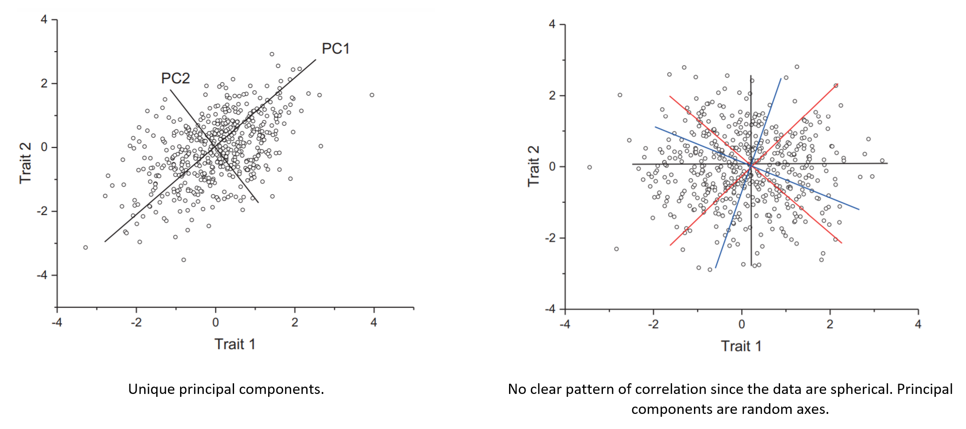
PCA is most effective when your features are correlated. It finds new axes that capture this shared information. If your features have no correlation, PCA can't do much. In such a case, the original feature axes are already the principal components.
The image below shows this contrast.
Conclusion
In this lesson, we have demystified Principal Component Analysis by focusing on its core objective. You've moved from the high-level need for dimensionality reduction to the specific mechanics of how PCA achieves it.
Key Takeaways:
- PCA's Goal: To transform a set of possibly correlated features into a new set of uncorrelated features called principal components.
- Variance Maximization: The primary objective of PCA is to find principal components that capture the maximum amount of variance in the data. PC1 accounts for the most variance, PC2 (orthogonal to PC1) for the second most, and so on.
- Two Perspectives: Maximizing the variance of the projected data is mathematically equivalent to minimizing the squared error between the original data and its projection.
- The Math Connection: The principal components are the eigenvectors of the data's covariance matrix. The corresponding eigenvalues measure the amount of variance captured by each principal component.
What's Next:
Now that you have a solid grasp of the theory behind PCA, the next step is to put it into action. In our next lesson, you will apply PCA to a high-dimensional dataset using Python's scikit-learn library. You will learn the most important part of the practical workflow: how to use the eigenvalues (or "explained variance") to decide how many principal components are needed to represent your data effectively.