Welcome back. In our previous lesson, we established a practical workflow for applying Principal Component Analysis and, most importantly, learned how to select the number of principal components to retain by analyzing the explained variance. We saw how to reduce dimensionality while preserving a desired amount of information.
Today, we will answer the crucial follow-up question: "Why is this useful?" This lesson connects the unsupervised technique of PCA directly to the world of supervised learning. You will learn how to use PCA as a powerful preprocessing step for a classifier, and we will rigorously evaluate its impact on both model performance and training efficiency. This is where the true value of dimensionality reduction in a machine learning pipeline becomes clear.
The Role of PCA in a Supervised Learning Pipeline
So far, we have treated PCA as a standalone data transformation technique. However, its most common application is as a preparatory step before feeding data into a supervised learning algorithm. There are several strategic advantages to this approach:
- Accelerated Training: With fewer features, model training can be significantly faster. For datasets with hundreds or thousands of features, the time saved can be substantial, enabling more rapid experimentation.
- Curse of Dimensionality Mitigation: In very high-dimensional spaces, data points become sparse, and the concept of distance can become less meaningful. This can degrade the performance of algorithms that rely on distance calculations, such as K-Nearest Neighbors. By projecting the data into a lower-dimensional space, PCA can make these algorithms more effective.
- Noise Reduction: By design, PCA prioritizes components that capture the most variance (the "signal") and discards those with low variance, which often correspond to noise. This can sometimes lead to a model that generalizes better to new, unseen data.
- Addressing Multicollinearity: Models like Linear and Logistic Regression can be sensitive to highly correlated features. Because principal components are orthogonal (uncorrelated) to each other, using them as input features completely eliminates multicollinearity.
Building an Integrated Workflow with scikit-learn Pipelines
When combining preprocessing steps (like scaling and PCA) with a final model, it is crucial to avoid data leakage. This means that any parameters learned during preprocessing (e.g., the mean/std from StandardScaler, or the principal components from PCA) must be learned only from the training data. These learned transformations are then applied to the validation and test sets.
Managing this manually can be error-prone. The scikit-learn Pipeline object is the standard, elegant solution. It chains together multiple steps—transformers and a final estimator—into a single object that behaves like a standard scikit-learn model.
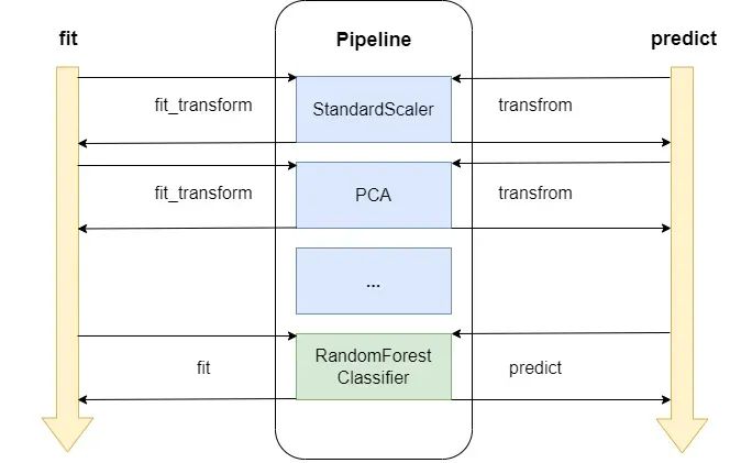
The following resource provides a clear introduction to the Pipeline API, which is a cornerstone of robust machine learning workflows in Python.
Component Analysis for Dimensionality Reduction in Python
This article from Machine Learning Mastery introduces the PCA API in scikit-learn and quickly pivots to showing how to integrate it into a Pipeline.
Please read the section titled PCA Scikit-Learn API. Focus on the syntax for creating a Pipeline object that chains transformers (like MinMaxScaler or PCA) with a final estimator (like LogisticRegression). This structure is what we will use for our experiment.
A Practical Experiment: PCA's Impact on a Classifier
Let's put this into practice with a concrete experiment. We will use the handwritten digits dataset, which is high-dimensional (64 features per image), making it a perfect candidate for PCA. Our goal is to train a LogisticRegression classifier and compare its performance and training time with and without PCA as a preprocessing step.
The following video from codebasics walks through this exact process. It establishes a baseline performance and then shows what happens after PCA is introduced.
Machine Learning Tutorial Python - 19: Principal Component Analysis (PCA) with Python Code
This video provides a step-by-step walkthrough of using PCA on the digits dataset, directly comparing the results of a logistic regression model before and after dimensionality reduction.
Please watch the following segments: Baseline Model: Observe the process of loading the data, scaling it, and training a LogisticRegression model on all 64 features. Note the final accuracy score (~97%) as our baseline. Applying PCA: Here, PCA is applied with n_components=0.95. This is the method we learned in the last lesson, where we ask scikit-learn to retain 95% of the variance. Notice how the number of features is reduced from 64 to 29. Model After PCA: A new LogisticRegression model is trained on the 29 principal components. Pay close attention to the final accuracy. It's nearly identical to the baseline, demonstrating that we lost very little predictive power despite discarding over half the features. The Trade-off: This final segment shows what happens when you are too aggressive with dimensionality reduction (e.g., n_components=2). The accuracy drops significantly, highlighting the trade-off between dimensionality and performance.
Quantifying the Impact: Performance and Training Time
The video showed that we can drastically reduce the number of features with minimal impact on accuracy. But what about the other key benefit: training speed?
Let's look at a more formal analysis that measures both accuracy and training time. The following guide uses the larger MNIST digits dataset (784 features) and explicitly measures the time it takes to fit a logistic regression model.
This tutorial from Built In provides a complete workflow for using PCA as a preprocessing step and includes a table that quantifies the reduction in training time.
Please read the section PCA to Speed-Up. This walks through the full process: loading data, splitting, scaling, applying PCA (again with a 95% variance threshold), and training a logistic regression model. Next, examine the table in the following section, Testing the Time. This table is the key takeaway. It clearly shows that as the variance retained (and thus the number of components) decreases, the model fitting time drops dramatically. Training with all features took nearly 2 minutes, while training on components representing 85% of the variance took only 10 seconds. This is a massive improvement in efficiency.
Finding the Sweet Spot: Components vs. Accuracy
We've seen that too few components hurt accuracy, while too many diminish the speed benefits. This implies there is an optimal range for the number of components. A common practice is to systematically evaluate model performance across a range of n_components to find this "sweet spot."
The plot below shows exactly this. The top panel is the scree plot showing the variance explained by each component. The bottom panel plots the classification accuracy of a model as a function of the number of principal components used for training.
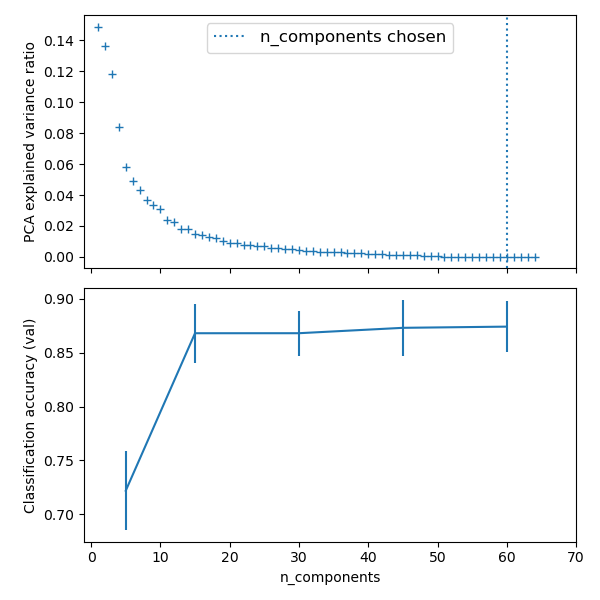
As you can see, the accuracy improves significantly as we add the first ~15 components, after which the gains become marginal. This analysis suggests that using around 15-20 components would provide a great balance of high accuracy and reduced dimensionality.
The machinelearningmastery.com article we looked at earlier demonstrates exactly how to generate a plot like this. It involves creating a loop to test a pipeline with a different number of components in each iteration.
Component Analysis for Dimensionality Reduction in Python
This article provides a runnable example for systematically evaluating the impact of component count on model performance.
First, quickly review the section Worked Example to see the setup of a Pipeline with a fixed n_components=10 and its evaluation using cross-validation. Then, focus on the code in the next section, which starts just after the reported accuracy. Read from How do we know. This section presents code that iterates from 1 to 20 components, evaluates the model at each step, and plots the results. The resulting box plot is analogous to the line chart we saw above, clearly showing performance saturating after a certain number of components.
This systematic evaluation is a robust way to justify your choice of n_components in a supervised learning context, moving beyond just the explained variance threshold.
Conclusion
In this lesson, you've integrated PCA into a supervised learning workflow, a crucial skill for handling high-dimensional data efficiently. You now understand not just how to apply PCA, but why and when it is a valuable tool in your preprocessing toolkit.
Key Takeaways:
- PCA as a Preprocessing Tool: PCA can significantly speed up model training, help mitigate the curse of dimensionality, and reduce noise by focusing on high-variance components.
- The
Pipelineis Essential: Usingscikit-learn'sPipelineis the standard and safest way to chain PCA with a classifier, as it prevents data leakage by properly fitting transformers on training data only. - Evaluating the Impact: The effectiveness of PCA is measured by a trade-off. We evaluate its impact on both training time (which should decrease) and model performance (which should remain high).
- Finding the Optimal Number of Components: You can systematically test different numbers of components and plot the resulting model accuracy to find a sweet spot that balances performance and computational efficiency.
What's Next:
PCA is a linear technique, meaning it captures linear relationships between features. But what if the underlying structure of your data is highly non-linear? In our next lesson, we will explore t-SNE (t-Distributed Stochastic Neighbor Embedding), a powerful non-linear technique primarily used for data visualization. We will contrast its purpose and mechanics with PCA to understand when to use each.