Welcome to our next lesson in feature engineering. In the previous lesson, we explored variance thresholding, a technique for removing features that have little to no variation and are therefore uninformative on their own. We learned that by looking at features in isolation, we can clean our dataset and reduce its complexity.
Today, we'll shift our perspective from individual features to the relationships between them. While a feature might be informative on its own, its value can be diminished if it provides the same information as another feature. This redundancy is what we'll tackle in this lesson. We will focus on correlation analysis, a powerful filter method for identifying and removing features that are highly correlated with one another, a condition known as multicollinearity. This step is crucial for building simpler, more stable, and often better-performing models.
The Problem of Multicollinearity
In the last lesson, our guiding principle was that a feature that doesn't change much offers little information. Today's principle is: a feature that changes in lockstep with another feature offers redundant information. When two or more independent variables in your dataset are highly correlated, it leads to a problem called multicollinearity.
Why is this a problem?
- Redundancy: Highly correlated features carry overlapping information. Including them all adds complexity to the model without adding new insight, potentially violating the principle of parsimony (Occam's razor).
- Model Instability: For certain models, particularly linear models, multicollinearity makes the model coefficients unstable. A small change in your training data can lead to drastic swings in the estimated coefficients for the correlated features. This makes it difficult to interpret the model and trust the importance it assigns to each feature.
- Overfitting: Some algorithms might place undue importance on a set of highly correlated features, leading to a model that performs well on training data but fails to generalize to new, unseen data.
The following video provides an excellent and intuitive mathematical explanation of how multicollinearity makes model coefficients unreliable.
The A to Z of Multicollinearity | Variance Inflation Factor | Data Preprocessing | Data Science
This video from the Six Sigma Pro SMART channel breaks down the concept of multicollinearity and visually demonstrates why it leads to unstable model coefficients, which directly addresses your goal of understanding the "why" behind these techniques.
Watch the segment from this explanation. The presenter uses a simple algebraic substitution to show how three different, yet equally valid, regression equations can emerge from the same data when features are correlated. This clearly illustrates the confusion it creates for the model.
For a supplementary textual definition, you can refer to the following article.
Detecting and Remedying Multicollinearity in Your Data Analysis
This article from Hex provides a concise written definition of multicollinearity and summarizes its consequences for model interpretability and performance.
Read the introduction and the section on the consequences. This will reinforce the concepts you just saw in the video.
Detecting Correlation
To deal with multicollinearity, we first need to detect it. The primary tools for this are the correlation matrix and its visualization, the heatmap. There are different types of correlation coefficients, but the most common for this task is the Pearson correlation coefficient, which measures the linear relationship between two numerical variables. It ranges from -1 (perfect negative correlation) to +1 (perfect positive correlation), with 0 indicating no linear correlation.
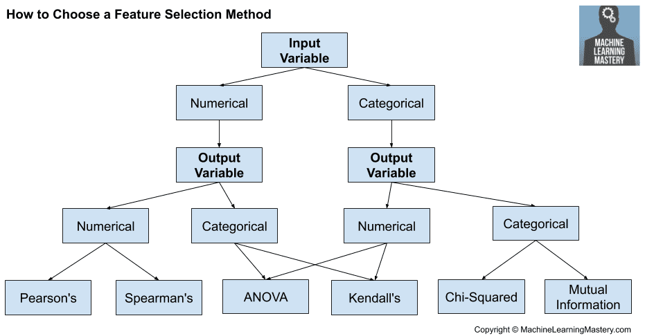
In Python, you can easily compute the pairwise correlation of all columns in a pandas DataFrame using the .corr() method. However, a table of numbers can be difficult to interpret, especially with many features. A heatmap provides an immediate, visual summary of the correlation matrix, using color intensity to represent the strength of the correlations.

A Systematic Approach to Removing Correlated Features
Once we have our correlation matrix, we need a systematic way to remove redundant features. The general algorithm is as follows:
- Calculate the absolute correlation matrix: We care about the strength of the correlation, not its direction (positive or negative). A correlation of -0.9 is just as redundant as +0.9.
- Use the upper triangle: The correlation matrix is symmetric (corr(A,B) = corr(B,A)). To avoid considering each pair twice, we only look at the values in the upper triangle of the matrix. We also ignore the diagonal of 1s.
- Set a threshold: Define a correlation threshold above which features will be considered highly correlated. Common values are 0.8, 0.85, or 0.9. This is a hyperparameter you can tune.
- Identify and drop features: Iterate through the correlation matrix and identify one feature from each pair whose correlation is above the threshold. Add these features to a "to_drop" list and remove them from the dataset.
As always, this process must be done after the train-test split and based only on the training data to prevent data leakage. The set of features identified for removal from the training set is then used to remove the same features from the test set.
The following video demonstrates this entire process practically.
Tutorial 2- Feature Selection-How To Drop Features Using Pearson Correlation
In this tutorial, Krish Naik provides a complete, hands-on walkthrough of using Pearson correlation for feature selection in Python.
First, watch the conceptual overview from this section, where he clarifies that we are concerned with correlations between independent features, not between an independent feature and the target variable. Next, pay close attention to the segment from the workflow setup. He correctly emphasizes performing the train-test split before any correlation analysis to prevent overfitting. Watch the demonstration from calculating correlation, where he uses x_train.corr() and seaborn.heatmap() to generate the correlation matrix and visualize it. Finally, watch the core logic from the removal function. He implements a function that iterates through the correlation matrix, applies a threshold, and identifies a set of features to be dropped.
The code in the video provides a robust and reusable function for this task. For a text-based version of the same logic, you can study the following guide.
How to Drop Out Highly Correlated Features in Python? - ProjectPro
This article from ProjectPro provides a step-by-step Python recipe for identifying and removing highly correlated features. It mirrors the logic you saw in the video.
Start by reading the introduction for a quick recap. Then, focus on the code implementation. Study Step 3, which shows how to get the correlation matrix and select the upper triangular part. Next, review Step 5, which contains the list comprehension logic to identify columns to drop based on a threshold. The code snippet under "Dropping columns" neatly summarizes this entire process.
Beyond Simple Removal: Other Techniques
While dropping a feature is the most direct way to handle multicollinearity, it's worth knowing about other approaches, some of which we will cover in detail later in this course.
- Variance Inflation Factor (VIF): VIF is a more formal statistical method to measure multicollinearity. For each feature, it runs a linear regression using all other features as predictors. The resulting R-squared value tells us how much of that feature's variance is explained by the other features. A high VIF score (typically > 5 or 10) indicates high multicollinearity. VIF-based elimination is often done recursively, removing the feature with the highest VIF score one at a time until all remaining features are below the threshold.
- Principal Component Analysis (PCA): Instead of dropping features, PCA combines the correlated features into a smaller set of new, uncorrelated variables called principal components. This is a dimensionality reduction technique that can resolve multicollinearity while retaining most of the information. We will dedicate a future lesson to PCA.
- Regularization: Certain machine learning models, like Ridge Regression, have built-in mechanisms that are robust to multicollinearity. Ridge regression adds a penalty to the model's cost function that shrinks the coefficients of correlated predictors towards each other, making the model more stable. This will be covered in the module on regularized linear models.
Conclusion
You have now learned another essential feature selection technique. While variance thresholding helps you remove features that are uninformative in isolation, correlation analysis helps you remove features that are redundant because they provide overlapping information.
Key Takeaways:
- Multicollinearity: A state where two or more independent variables are highly correlated. It can make models unstable and difficult to interpret.
- Detection: Use a correlation matrix (
.corr()) and a heatmap (seaborn.heatmap()) to visualize relationships between features. - Remediation: The most common method is to set a correlation threshold (e.g., 0.85) and systematically remove one feature from any pair that exceeds this threshold.
- Workflow: Always perform correlation analysis after the train-test split and derive the features to drop from the training set only. Apply the removal to both train and test sets.
- Scope: This method is primarily for linear relationships between numerical features. The absolute value of the correlation is what matters.
In our next lesson, we will put everything together. You will apply a complete preprocessing pipeline to a raw, real-world dataset, combining the skills you've learned for exploratory data analysis, data cleaning, encoding, scaling, and feature selection into a single, cohesive workflow.