In our previous lesson, we explored univariate analysis, learning how to examine variables one by one using histograms, density plots, and box plots. This gave us a solid foundation for understanding the individual characteristics of our data. Now, we will build on that by moving into the exciting realm of bivariate and multivariate analysis, where we investigate the relationships between variables.
Understanding how variables interact is a cornerstone of machine learning. It helps us identify predictive features, detect redundancy, and build more effective models. In this lesson, you will learn to visualize these relationships using three powerful tools from the seaborn library: scatter plots, correlation heatmaps, and pair plots. By the end, you'll be able to create and interpret these visualizations to uncover the hidden connections within your data.
The Scatter Plot: Visualizing Two-Variable Relationships
The most fundamental tool for exploring the relationship between two continuous variables is the scatter plot. Each point on the plot represents a single observation (a row in your dataset), positioned according to its values on the two variables assigned to the X and Y axes.
When interpreting a scatter plot, we look for three key characteristics:
- Direction: Is the relationship positive (as one variable increases, the other tends to increase) or negative (as one increases, the other tends to decrease)?
- Strength: How closely do the points follow a clear pattern? A tight cluster of points suggests a strong relationship, while a diffuse cloud suggests a weak one.
- Form: Is the relationship linear (forming a straight line) or non-linear (forming a curve)?
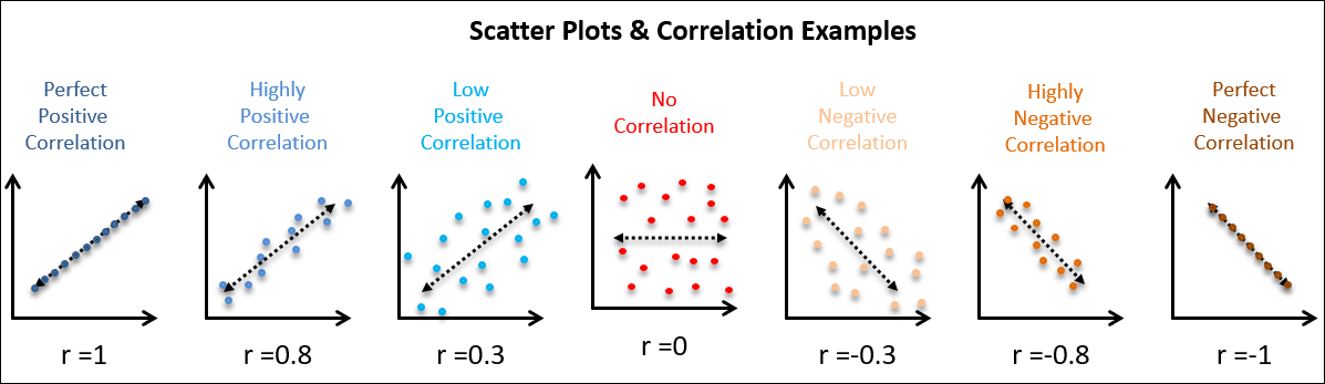
The image below illustrates several examples, along with the Pearson correlation coefficient (r), a value between -1 and 1 that measures the strength and direction of a linear relationship. A value of 1 indicates a perfect positive linear relationship, -1 a perfect negative linear relationship, and 0 no linear relationship.
Given your proficiency in Python, you'll find creating these plots with seaborn to be intuitive. A great feature of seaborn is the ability to add more dimensions to a plot using visual cues like color (hue), marker style (style), and size (size).
The following video provides a thorough walkthrough of creating and customizing scatter plots with seaborn, covering everything from basic syntax to encoding additional variables.
Seaborn scatter plot | How to make and style a scatterplot in Python seaborn
This tutorial by Kimberly Fessel offers a detailed guide to seaborn.scatterplot, which is the primary function for this task.
Watch the beginning to understand the basics of scatter plots and the two main ways to pass data to the function. Next, focus on the section explaining how to add more information using the hue, style, and size parameters. This is key for multivariate visualization. Finally, review the section on advanced styling, which covers transparency (alpha) and other customization options that are useful for dense plots.
From Visuals to Numbers: The Correlation Matrix
While scatter plots are excellent for visualizing relationships, we often need a quantitative summary, especially when dealing with many features. This is where the correlation matrix comes in. It's a square table that shows the correlation coefficient for every pair of numerical variables in your dataset.
Before we learn how to create one, it's important to understand its properties and what correlation truly represents. The following article provides an excellent conceptual breakdown.
Correlation matrix, demystified
This article from Towards Data Science clearly explains the concept of a correlation matrix, its mathematical properties (in an intuitive way), and how it's constructed from a dataset.
First, read the introductory section on correlation. Pay close attention to the crucial distinction between correlation and causation. Next, read the section on the correlation matrix itself. This explains its key properties, such as being square, symmetric, and having 1s on the diagonal. Finally, read the section on building a correlation matrix. This walks through the logic of how variables are mapped to the rows and columns of the matrix.
The Heatmap: Visualizing the Correlation Matrix
A correlation matrix can be dense and difficult to interpret, especially with many variables. It's just a grid of numbers. A heatmap solves this by representing the matrix graphically, using color to convey the magnitude and direction of the correlations. This allows you to spot strong positive or negative correlations at a glance.
In seaborn, you can generate a correlation matrix from a pandas DataFrame using the .corr() method and then pass it directly to the seaborn.heatmap() function.
The following video demonstrates this process and shows why heatmaps are so effective for exploratory analysis.
Seaborn Is The Easier Matplotlib
This video from the NeuralNine channel (which you saw in the last lesson) has an excellent segment on heatmaps. The presenter rightly calls it one of the most important plots for data exploration.
Watch the section that explains and demonstrates how to create and interpret a correlation heatmap. Notice how quickly you can identify the most and least correlated features by looking at the colors.
The Pair Plot: A Bird's-Eye View of Relationships
What if you want to quickly inspect the relationships between all numerical variables in your dataset without creating dozens of individual scatter plots? The pair plot (sometimes called a scatter plot matrix) is the perfect tool for this.
A pair plot creates a grid of axes such that each variable in your data is shared across a single row and a single column. This results in two types of plots:
- Off-diagonal: Scatter plots for every pair of variables.
- Diagonal: A univariate plot (typically a histogram or density plot) for each variable, showing its distribution.
This single visualization gives you a comprehensive overview of both the pairwise relationships and the individual distributions of your variables, elegantly combining the topics from this lesson and the previous one.

Creating a pair plot is remarkably simple with seaborn. The following reading shows you how.
Visualizing Data with Seaborn in Python: A Beginner-to- ...
This guide from Udacity provides clear, concise code examples for the plots we've discussed today.
Review these three sections to see the Python code in action: Read the section on Scatter Plots for a quick code reference. Next, read about Heatmaps to see how to generate a correlation heatmap from scratch. Finally, read the section on the Pairplot, which demonstrates how to create this powerful summary visualization with a single line of code.
Summary of Key Takeaways
In this lesson, we moved from analyzing single variables to exploring the rich web of relationships between them. This is a critical step in understanding your data and preparing it for machine learning.
- Scatter Plots: These are your go-to for visualizing the relationship between two numerical variables. You can add more dimensions using
hue,style, andsize. - Correlation Matrix & Heatmap: The correlation matrix quantifies the linear relationships between all pairs of variables. A heatmap provides an immediate visual summary of this matrix, making it easy to spot strong correlations. Remember: correlation does not imply causation.
- Pair Plots: This powerful tool gives you a holistic view of your dataset by combining pairwise scatter plots with univariate distribution plots for every variable, all in one visualization.
You now have a complete set of fundamental tools for both univariate and bivariate exploratory data analysis.
In our next lesson, we will apply these visualization skills to a crucial task in data cleaning: identifying data quality issues such as missing values and outliers. The patterns you've learned to spot today will be your guide.